Editor: Plot Tool ()
The Plot Tool is a special-purpose viewer designed to display 1-dimensional data, e.g., function curves. Instead of being a separate module, the Plot Tool is invoked implicitly by certain modules such as the data probing modules (Point Probe, Line Probe, and Spline Probe) or the Multi-Thresholding module. Each of these modules generates 1-dimensional data such as a function plot along a line or a histogram. For most of these modules it is possible to display the plot within 's viewer if one connects the Plot In Viewer module to it. While the data-generating modules control the initial settings of the plot window, the user can freely adjust these settings afterwards.
Plot Basics
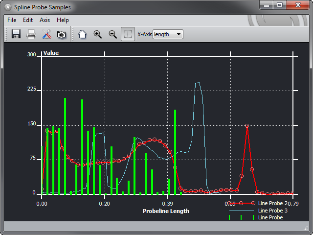
Figure 1: 's plot window. The layout of the plot is determined by objects and groups of objects. These entities are processed by a plot engine. In particular, there are objects for
- Curves
- Cartesian axes
- Polar axes
- Plot areas
- Legends
- Annotations
- Marker lines
- Lattices
- Colormaps
The plot engine processes the objects top to bottom (see Figure below). The sequence of objects determines their behavior. Objects of type PlotArea define the area within the plot window where objects are placed. This area is given in normalized coordinates with the origin at the lower left corner. Besides this, a PlotArea object also acts as a grouping object. An axis is placed in such an area and establishes, together with the preceding PlotArea, a window-viewport (world coordinates to normalized coordinates) transformation. Note that the objects must be kept in the following sequence: 1. PlotArea, 2. Axis, 3. Curves and Marker lines. Legends display all succeeding curves in the sequence and can be placed wherever needed. It is possible to have more than one plot area or axis in a plot setup.
Every object is identified by a unique name. You will need to know these names if you want to change certain object attributes via the command interface of the Plot Tool.
Editing Parameters
In order to change the parameters of a plot object, select the Edit Objects... item from the Edit pulldown menu of the Plot Tool. A window appears with the list of names of all objects currently in use. When you select one of these objects, the parameters of that object are displayed and can be changed. The is active toggle near the lower left corner of the window can be used to switch the processing of the selected object on or off. If the processing of an object which has group functionality (Plot Areas, Plot Groups) is switched off, all objects within that group are also not processed.
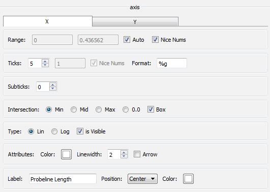
Figure 2: Dialog for editing plot objects. On the right hand side the controls for editing axis parameters are shown. The following sections document all parameters that are not self-explanatory.
Editing axis parameters
To choose the x- or y-component of an axis, just click on the appropriate tab. If you want to change the range, you must switch off the Auto toggle. This causes the range fields to become sensitive. The Nice Num toggle sets the range to the next "good looking" boundaries. A tick delta can be typed in after the number of ticks is set to -1.
It is possible to zoom interactively into your data using the mouse. To do this, drag a rectangle within the plot area by pressing the shift key and the left mouse button while moving the mouse. To go back to the automatic ranges, click into the plot area with the left mouse button while the Alt key is pressed at the same time.
Every axis object has a hidden grid child object which is not active by default. To show the grid, just open the grid child and select it. Then set the is active toggle to on.
Editing annotation parameters
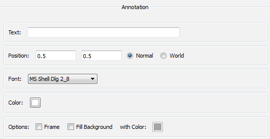
Figure 3: Editable annotation parameters. To position an annotation on your plot, you can switch between world coordinates or normalized coordinates. Using world coordinates is convenient if you want to annotate a certain feature, e.g., an extrema of a curve. In this case, you must insert the annotation after that curve object. You can also position an annotation in the plot window interactively by pressing the left mouse button on the annotation, moving the mouse, and then releasing it at the new position.
Editing legend parameters
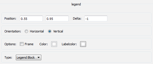
Figure 4: Editable legend parameters. There are three types of legends possible: A Legend Block displays an entry for each curve together with a short line depicting the appearance of the curves. A Name Block is just a list of the curve names. The position and orientation for both types can be manipulated easily in the editor window. The position denotes the coordinates of the first legend item. Positions of legends are always normalized coordinates. The delta parameter applies only to the vertical (y) coordinate. You can also position a legend in the plot window interactively by pressing the left mouse button on one of the names in the legend, moving the mouse, and releasing it at the desired position. The third legend type (Name List) displays a list of curve names, too. But in contrast to the latter type, you can move every name around separately, like you can with annotations (see above).
Editing marker line parameters
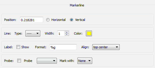
Figure 5: Editable marker line parameters. The position of a marker line must be given in world coordinates. Also be sure that the marker line is inserted after the appropriate axis. You can shift a marker line horizontally or vertically in the plot window by pressing the left mouse button on the marker line, moving the mouse, and releasing it at the new position. Marker lines can be used to probe those curves which belong to the same group (PlotArea) as the marker line. You can display the value where the marker line intersects the selected curve the first time. This intersection can also be indicated with a marker symbol.
Editing lattice parameters
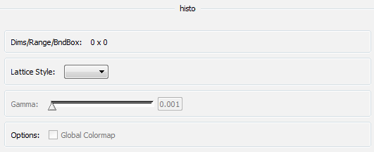
Figure 6: Editable lattice parameters. A lattice is a two-dimensional field which is rendered as an image by default. If both dimensions are less than or equal to 32, a lattice can also be rendered as colored dots in a grid (Gridded) or as dots of different sizes (Spot) to represent the values. For lattices rendered as images, a gamma value can be set to enhance the image. Lattices have a colormap (Default: black to white) which can be set through the appropriate modules. Global colormaps are not supported within .
Editing colormap parameters

Figure 7: Editable colormap parameters. Colormaps have only a few editable parameters: The minimum and maximum values can be given or taken from the axis if there is one. Furthermore the colormap can be reversed. The colors itself can only be changed with the colormap editor.
Editing (analytical) curve parameters
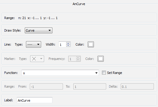
Figure 8: Editable (analytical) curve parameters. Besides the more or less self-explanatory parameters of both the curve and analytical curve (AnCurve) parameters, there are a few things to mention regarding AnCurves only. The Function text widget contains the formula which is computed on every plot update. The default formula is x, which produces a transversal line where x runs from -1 to 1. It is possible to use the name of another curve as a variable in the function. In this case, the x-values of the first curve in the formula are taken to evaluate the y-values of all variables in use. These y-values are then used for the computation. You can restrict the range of the computation by activating the Explicit Range toggle and entering the appropriate range values. There are many built-in functions such as sin, cos, tan, sqrt, exp, ... which can be used in formulas.
Working with Plot Objects
You can copy or delete plot objects. For example, it may be useful for comparison purposes to copy a curve before the data of the original curve will be changed. To do so, you must select the object in the list and then choose the Edit/Copy pulldown menu. After that, choose Paste or Append in the menu and the object will be inserted at the current position (= position of the selected object) or the object will be placed behind the selected object.
With the New pulldown menu you can create new objects which will be inserted at the appropriate positions in the list of objects.
Printing
The File pulldown menu of the main plot window provides a Snapshot item where you can send the plot directly to the default printer or save it as an image file. It is also possible to generate a vector-based PostScript file of the plot by using the print command (see below).
Saving Data
The Save Data... item under the File menu lets you save the data of all curves in a file. The file dialog presents a list of formats suitable for saving the data.
Data formats
The Plot (.ampl) is a proprietary format which should be used if you want to plot the data later on within the plot facilities. Use the Gnuplot (.dat) if you plan to use Gnuplot to plot the data outside of . If you need to import the plot data into a spreadsheet program like Microsoft's Excel, use the CSV (CSV = Comma Separated Values) (.csv). The ascii (.am) can be loaded and processed by .
Saving the Plot State
If you changed your plot setup a lot, you can save this setup in a similar fashion like the Save Project functionality. That is, first save the project, and then save the plot state into a second file. To resume an session, invoke and load the two script files (1. project, 2. Plot state). Note that the size and the position of a plot window is saved automatically if it is opened by an module and the Save Project menu item is invoked.
Specific Options
For the Spline Probe and Line Probe, a specific plot toolbar is available that let you choose the X axis type:
- Length : The X axis represents the length of the curve (default).
- x-coord : The X axis represents the X coordinate of the curve sampled points.
- y-coord : The Y axis represents the Y coordinate of the curve sampled points.
- z-coord : The Z axis represents the Z coordinate of the curve sampled points.
For HxLabelAnalysis spreadsheets (generated for example by Label Analysis and Analysis Filter modules), another specific plot toolbar is available.

Figure 9: Label Analysis spreadsheet toolbar
- The drop-down list allows selecting the column of the analysis to plot. In case of spreadsheet created by Label Analysis module, the list consists of the spreadsheet's measures.
- The gear button allows opening the Histogram Parameters dialog:
- The Cumulative option allows switching from a ordinary to a cumulative histogram.
- If Normalized option is selected, the bins' values will be normalized either between 0 and 1, or between 0 and 100 percents.
- Number of bins gives the number of bins to display.
- If Logarithmic scaling option is selected, a logarithmic scaling will be used on the vertical axis.
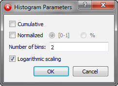
Figure 10: Histogram Parameters dialog
In , Plot Tool commands have the following structure:
$thePlot command [ parameters ]
or if the command applies to a plot object:
$thePlot objectname command [ parameters ]
The following general commands are available:
getSize
Returns the size of the plot window.setSize <width> <height>
Sets the size of the plot window.getPosition
Returns the position of the plot window relative to the upper left corner of the screen.setPosition <x> <y>
Sets the position of the plot window relative to the upper left corner of the screen.setBackgroundColor <r> <g> <b>
This command sets the color of the background to a specific value. The color may be specified either as a triple of integer RGB values in the range 0...255, as a triple of rational RGB values in the range 0.0...1.0, or simply as plain text, e.g., white, where the list of allowed color names is defined in /usr/lib/X11/rgb.txt.hide
Hides the plot window.show
Shows the plot window if it is hidden.getObjects
Displays a list of all plot objects currently in use.update
Processes the plot object and updates the display.snapshot <filename>
Takes a snapshot and saves it under the given name. The suffix of the filename determines the raster format used. Available formats are: TIFF (.tif,.tiff), SGI-RGB (.rgb,.sgi,.bw), JPEG (.jpg,.jpeg), PNM (.pgm,.ppm), BMP (.bmp), PNG (.png), and Encapsulated PostScript (.eps)print [options] <filename>
Prints the plot window into a PostScript file (vector based) with the following options:-a4 : generates a4 landscape output (Default).
-a5 : generates a5 portrait output.
-auto : switches autoscaling on (Default).
-bw : generates black and white output.
-color : generates color output (Default).
-eps : generates encapsulated PostScript.
-fillbg : fills the background according to the plot window.
-frame : draws a frame around the plot.
-landscape : prints in landscape format.
-noauto : switches autoscaling off.
-portrait : prints in portrait format.
-windowsize : generates output of window size.saveData <filename>
Saves the data of all data based plot objects in a proprietary format.saveState <filename>
Saves the current plot state into a script file that can be used to restore the plot setup in a future session.load <filename>
Loads data from the filename and stores it in a curve plot object.setXAxisType <type>
Sets the X axis type. Available types are:
- length : The X axis represents the length of the curve (default).
- xcoord : The X axis represents the x coordinate of the curve sampled points.
- ycoord : The X axis represents the y coordinate of the curve sampled points.
- zcoord : The X axis represents the z coordinate of the curve sampled points.
This command is available only for the Spline Probe and Line Probe.
The following commands apply to plot objects:getMinMax
Returns the minimum and maximum values of objects of type: Curve, Cartesian Axis, Polaraxis.setMinMax <minX> <maxX> <minY> <maxY>
Sets the range of Cartesian Axis, Polaraxis.getArea
Returns the plotting area of PlotArea objects.setArea <lowerleftX> <lowerleftY> <upperrightX> <upperrightY>
Sets the plotting area of a PlotArea object.getXValues
Returns the x-values of a Curve.getYValues
Returns the y-values of a Curve.set[X|Y|Phi|R]TickValues <tick1> <tick2> ... <tickN>
Sets the position of the ticks along an axis. It is available for objects of type: Cartesian Axis, Polaraxis.set[X|Y|Phi|R]TickLabels <label1> <label2> ... <labelN>
Sets the labels of the ticks along an axis. It is available for objects of type: Cartesian Axis, Polaraxis. If there are fewer labels than ticks the remaining ticks will be unlabeled.