Module: 2D-Histogram Segmentation ()

Description:

Using the 2D-Histogram Segmentation script module, you can make the segmentation of your CT or MR gray level images data composed of two or more phases in a semi-automatic way.

References
The implementation of this segmentation is based on the following publication:
Assessment of bone ingrowth into porous biomaterials using MICRO-CT
Anthony C. Jones, Christoph H. Arns, Adrian P. Sheppard, Dietmar W. Hutmacher, Bruce K. Milthorped, Mark A. Knackstedt
Department of Applied Mathematics, Research School of Physical Sciences and Engineering, Australian National University, Canberra ACT 0200, Australia.

The method described in this paper has two steps:

1. Use a 2D scatter-plot (histogram) of Gradient Magnitude vs Intensity to select a seed region. We use the same step in the module implementation.
2. Use ANU's "Converging Active Contours" algorithm to expand the seed. In the module implementation, we use instead a watershed algorithm to expand the seed.

Introduction

Consider a multiphase material like the tutorial data chocolate-bar.am, a CT scan of the cylinder head sample. There are many discrete phases, but the histogram shows that the peaks from the differing phases overlap. In cases like this, thresholding the image based on intensity will fail because any threshold will result in some pixels being incorrectly assigned.

The approach used here, called 2D-Histogram Segmentation, relies on the Gradient Magnitude versus Image Intensity histogram.

This segmentation process includes two major steps: an initial classification of some voxels into two or more phases, and then a expansion step where that classification is expanded so that all voxels become labeled.

• Classification: For this routine the initial classification of voxels is performed based on those voxels' intensity and their gradient magnitude. The input to this routine is the intensity map of a 3D volume. From that input, the gradient magnitude is computed. Once the gradient magnitude is computed, the user is presented with a 2D scatterplot that shows Gradient Magnitude vs Image Intensity. The user will use this plot to determine the initial classification (this is described in Use the histogram to initialize the classification).
• Expansion: Expansion is computed by the marker-seeded watershed transform (see Principle of the watershed algorithm). The watershed transform requires two inputs, a set of seed markers and a landscape function. The seed markers will be determined by classification (see Interpreting the histogram), and the gradient magnitude will be used for the landscape function.

The 6 steps of the 2D histogram segmentation:

• Step 1 - Compute gradient magnitude to begin - see detail in Computing the gradient magnitude:
  Choose between precise computation of the gradient magnitude or a faster approximation of the gradient magnitude.
  Hit Next: Compute Gradient Magnitude to continue.
  
• Step 2 - Plot histogram see details in Interpreting the histogram:
  Hit Next: Plot Histogram to continue.
  
• Step 3 - Draw windows - see details in Use the histogram to initialize the classification:
  If you used the mouse to drag the plot window, and you wish to reset to its original size and position, you can simply drag the Gamma Correction slider on the Properties panel.
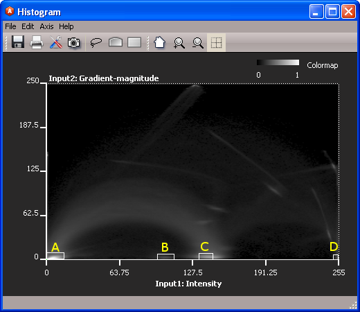
  Use gamma correction to visualize peaks on the 2D histogram. Use drawing tools at top of plot window to draw windows directly on the plot. Generally, you want to select regions that have very low gradient-magnitude (peaks close to the x axis).
  Hit Next: Compute Seed to proceed to the next step.
  
• Step 4 - Review seed labels:
  Use weight factor to update the view to show the grayscale data, the seeded label image, or a weighted fusion of the two data sets.

  Use the Hide/Show Histogram button to toggle the display of the histogram so that it is easier to view the results in the Viewer. Use slice number to adjust the slice index plane that is being displayed. If you are not satisfied with the seeds computed from your chose windows, hit Delete Last Window to delete windows one at a tie (in the reverse order from which they were added). Then you can draw new windows. After you have drawn new windows, hit Recompute Seed. You can iterate until you are satisfied with the seed.

  Hit Next: Apply Watershed to proceed (see details in Use watershed to expand)

• Step 5 - Confirm watershed results:
  If the results are not satisfactory, draw new regions, and then reapply watershed with hitting Previous: Recompute Seed.
  Hit Next to proceed to the final step, which is optional.
  
• Step 6 - [Optional] Delete a channel:
  If one of the assigned labels corresponds to void space, you may choose to delete that label from the label image.

  You should delete this module when you are done.

Computing the gradient magnitude - details of step 1
When you connect this module to an input data, you will have to choose for a precise or approximate (but faster) computation of the gradient magnitude. After the gradient magnitude is computed, a scatterplot will be generated that shows the Gradient Magnitude vs Image Intensity (see Figure 1). The scatterplot is computed and plotted using the Correlation Histogram modules.

Figure 1: Histogram of Gradient Magnitude vs Intensity

Interpreting the histogram - details of step 2
Low gradient-magnitude regions are generally unambiguous, and they can be definitively classified as material or another.

High gradient-magnitude regions are ambiguous, and may belong to either of two materials. These are voxels that fall on the boundary between two materials.

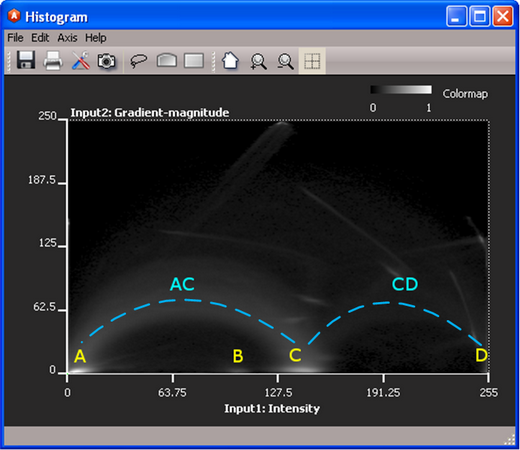
For each phase in your multiphase material, you should see a small cluster of high density pixels somewhere near the bottom of the histogram. The y-value of the cluster will be small, and the x-axis will correspond to the average intensity of that phase. For each pair of phases that share an interface, you will see an arc of density linking the two clusters; the arc will span higher gradient (y-axis) space.

Consider the histogram for chocolate-bar.am. chocolate-bar.am has three distinct materials: air, low-density metal, and high-density metal. The histogram shows four potential phases (A,B,C, and D), and it also reveals information about the boundaries between phases where you can see at least two connecting arcs (AC and CD). The absence of any arcs connecting B suggests that the B cluster may not be a real phase.

Figure 2: Same 2D Histogram as before, after adjusting the gamma function. Note the potential phase clusters (A, B, C, D) and the two phase interface arcs (AC and CD).

Use the histogram to initialize the classification - details of step 3

Figure 3: Four windows have been drawn to select the four prospective phase clusters.

Use the drawing tools to draw windows. Draw one window for each material (include A, B, C, and D).

After you have drawn one window corresponding to each material, hit Next: Compute Seed to visualize the voxels corresponding to the windows you have selected. The classification results are visualized on an Ortho Slice and its coupled Color Wash. The slider in the Weight factor port (on the Color Wash module) will allow you to adjust the weighting factor so you can slide between seeing the classified pixels or the grayvalue pixels.

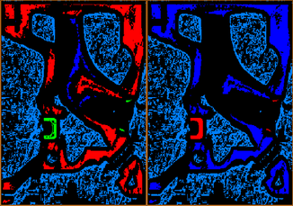
The first window you chose will be colored light blue, the second window royal blue, the third red, and the fourth green. By visual inspection, you can see that the royal blue pixels (corresponding to region B) are not a separate phase, but instead a region of blurred density connecting phases A and C; these are probably imaging artifacts related to the instruments modulation transfer function.

This process of visual inspection allows us to review the classification results, and then, if necessary, remove and recreate windows (use the Delete Last Window button to delete windows). The classification by the new windows can then be visualized. This iterative procedure is continued until you are satisfied by the classification results.

Figure 4: Left: Classification result of windows for A, B,C and D.Right: Classification results for windows A, C, and D.

Use watershed to expand - details of step 4
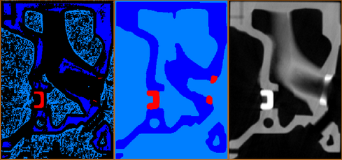
The second step is to perform a watershed transform. The watershed transform will expand the classified pixels and the result will be that all of the pixels will be classified according to one of the phases.

This is done for you automatically when you click on Next: Apply Watershed button.

Figure 5: Left: Results window-based classification.Middle: Results after watershed expansion.Right: Initial gray-value image.

Connections:

Data [required]
Image data to be segmented.

Ports:

Intensity

Displays information on the input gray-level image.

GradientMagnitude

Displays information on the computed gradiant magnitude.

Visibility

This port is only displayed at the step 3, step 4, step 5 and step 6.
Controls the visibility of the histogram.

Slice number

This port is only displayed at the step 4, step 5 and step 6.
Adjusts the slice index plane that is being displayed.

Weight factor

This port is only displayed at the step 4, step 5 and step 6.
Choose the weight factor to update the view to show the grayscale data, the seeded label image, or a weighted fusion of the two data sets.

Colormap

This port is only displayed at the step 4, step 5 and step 6 and chooses the colormap to use for displaying seeds and segmented image.

Next action

Displays information concerning the next action to come and the current step.

Gradient method

This port is only displayed at the step 1 and chooses the method to use to compute the gradient magnitude.

Gamma correction

This port is only displayed at the step 3, step 4, step 5 and step 6.
Chooses the gamma correction to apply to the histogram.

Delete channel

This port is only displayed at the step 6 and enables deleting a specific channel which corresponds to void space.

Action



Proposes the different actions to apply. At each step, the list of actions is updated.