Distributed Radar Tracking Simulation

This example uses the Parallel Computing Toolbox™ to perform a Monte Carlo simulation of a radar station that tracks the path of an aircraft. The radar station uses the radar equation to estimate the aircraft position. We introduce measurement errors as a random variable, and the radar station performs Kalman filtering to try to correct for them. To estimate the effectiveness of the Kalman filter, we perform repeated simulations, each time having the aircraft travel along a randomly chosen path.

For details about the computations, open the pctdemo_model_radar model open the pctdemo_model_radar model.

Prerequisites:

Related examples:

Sequential Radar Tracking Simulation

Analyze the Sequential Problem
Load the Example Settings and the Data
Divide the Work into Smaller Tasks
Create and Submit the Job
Retrieve the Results
Measure the Elapsed Time
Plot the Results

Analyze the Sequential Problem

First, we look at how the computations in the sequential example fit into the model introduced in the Dividing MATLAB Computations into Tasks example. The main computations consist of a large number of simulations, and each simulation takes only a fraction of a second. We therefore have each task perform many simulations. Because the function pctdemo_task_radar can already perform many simulations in a single function call, we can use it directly as our task function.

Load the Example Settings and the Data

The example uses the default profile when identifying the cluster to use. The profiles documentation profiles documentation explains how to create new profiles and how to change the default profile. See Customizing the Settings for the Examples in the Parallel Computing Toolbox for instructions on how to change the example difficulty level or the number of tasks created.

[difficulty, myCluster, numTasks] = pctdemo_helper_getDefaults();

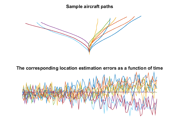
We define the number of simulations and the length of each simulation in pctdemo_setup_radar. The example difficulty level controls the number of simulations we perform. The function pctdemo_setup_radar also shows examples of the different paths that the aircraft can take, as well as the error in the estimated aircraft location. You can view the code for pctdemo_setup_radar view the code for pctdemo_setup_radar for full details.

[fig, numSims, finishTime] = pctdemo_setup_radar(difficulty);
startClock = clock;

Divide the Work into Smaller Tasks

The computationally intensive part of this example consists of a Monte Carlo simulation and we use the function pctdemo_helper_split_scalar to divide the numSims simulations among the numTasks tasks.

[taskSims, numTasks] = pctdemo_helper_split_scalar(numSims, numTasks);
fprintf(['This example will submit a job with %d task(s) ' ...
         'to the cluster.\n'], numTasks);

This example will submit a job with 4 task(s) to the cluster.

Create and Submit the Job

Let us create the simulation job and the tasks in the job. We let task i perform taskSims(i) simulations. Notice that the task function is the same function that you used in the sequential example. You can view the code for pctdemo_task_radar view the code for pctdemo_task_radar for full details.

job = createJob(myCluster);
for i = 1:numTasks
    createTask(job, @pctdemo_task_radar, 1, {taskSims(i), finishTime});
end

We can now submit the job and wait for it to finish.

submit(job);
wait(job);

Retrieve the Results

Let us obtain the job results, verify that all the tasks finished successfully, and then delete the job. fetchOutputs will throw an error if the tasks did not complete successfully, in which case we need to delete the job before throwing the error.

try
    jobResults = fetchOutputs(job);
catch err
    delete(job);
    rethrow(err);
end

Let us format the results. Notice how we concatenate all the arrays in jobResults along the columns, thus obtaining a matrix of the size (finishTime + 1)-by-numSims.

residual = cat(2, jobResults{:});

We have now finished all the verifications, so we can delete the job.

delete(job);

Measure the Elapsed Time

The time used for the distributed computations should be compared against the time it takes to perform the same set of calculations in the Sequential Radar Tracking Simulation example. The elapsed time varies with the underlying hardware and network infrastructure.

elapsedTime = etime(clock, startClock);
fprintf('Elapsed time is %2.1f seconds\n', elapsedTime);

Elapsed time is 34.4 seconds

Plot the Results

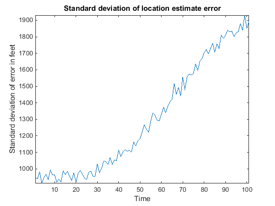
We use the simulation results to calculate the standard deviation of the range estimation error as a function of time. You can view the code for pctdemo_plot_radar view the code for pctdemo_plot_radar for full details.

pctdemo_plot_radar(fig, residual);

Was this topic helpful?

Documentation