Documentation

This example uses Conway's "Game of Life" to demonstrate how stencil operations can be performed using a GPU.

Many array operations can be expressed as a "stencil operation", where each element of the output array depends on a small region of the input array. Examples include finite differences, convolution, median filtering, and finite-element methods. This example uses Conway's "Game of Life" to demonstrate two ways to run a stencil operation on a GPU, starting from the code in Cleve Moler's e-book Experiments in MATLAB.

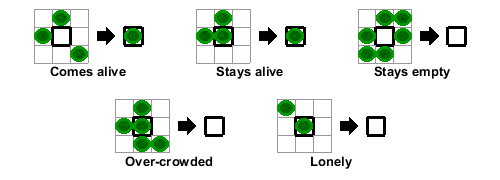
The "Game of Life" follows a few simple rules:

• Cells are arranged in a 2D grid

• At each step, the fate of each cell is determined by the vitality of its eight nearest neighbors

• Any cell with exactly three live neighbors comes to life at the next step

• A live cell with exactly two live neighbors remains alive at the next step

• All other cells (including those with more than three neighbors) die at the next step or remain empty

The "stencil" in this case is therefore the 3x3 region around each element. Here are some examples of how a cell is updated:

This example is a function to allow the use of nested functions:

function paralleldemo_gpu_stencil()

Generate a random initial population

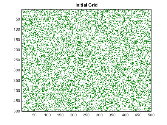
An initial population of cells is created on a 2D grid with roughly 25% of the locations alive.

gridSize = 500;
numGenerations = 100;
initialGrid = (rand(gridSize,gridSize) > .75);
gpu = gpuDevice();

% Draw the initial grid
hold off
imagesc(initialGrid);
colormap([1 1 1;0 0.5 0]);
title('Initial Grid');

Playing the Game of Life

The e-book Experiments in MATLAB provides an initial implementation that can be used for comparison. This version is fully vectorized, updating all cells in the grid in one pass per generation.

    function X = updateGrid(X, N)
        p = [1 1:N-1];
        q = [2:N N];
        % Count how many of the eight neighbors are alive.
        neighbors = X(:,p) + X(:,q) + X(p,:) + X(q,:) + ...
            X(p,p) + X(q,q) + X(p,q) + X(q,p);
        % A live cell with two live neighbors, or any cell with
        % three live neighbors, is alive at the next step.
        X = (X & (neighbors == 2)) | (neighbors == 3);
    end

grid = initialGrid;
% Loop through each generation updating the grid and displaying it
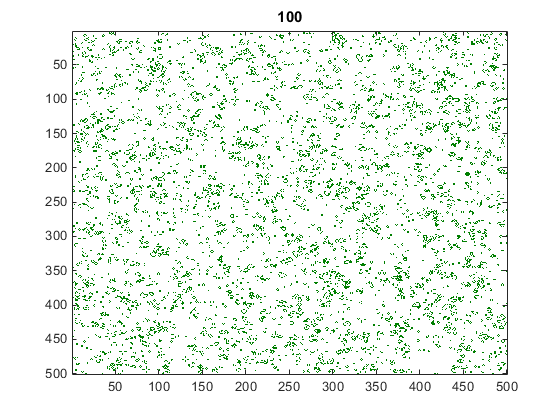
for generation = 1:numGenerations
    grid = updateGrid(grid, gridSize);

    imagesc(grid);
    title(num2str(generation));
    drawnow;
end

Now re-run the game and measure how long it takes for each generation.

grid = initialGrid;
timer = tic();

for generation = 1:numGenerations
    grid = updateGrid(grid, gridSize);
end

cpuTime = toc(timer);
fprintf('Average time on the CPU: %2.3fms per generation.\n', ...
    1000*cpuTime/numGenerations);

Average time on the CPU: 11.323ms per generation.

Retain this result to verify the correctness of each version below.

expectedResult = grid;

Converting the Game of Life to run on a GPU

To run the Game of Life on the GPU, the initial population is sent to the GPU using gpuArraygpuArray. The algorithm remains unchanged. Note that wait(gpu)wait(gpu) is used to ensure that the GPU has finished calculating before the timer is stopped. This is required only for accurate timing.

grid = gpuArray(initialGrid);
timer = tic();

for generation = 1:numGenerations
    grid = updateGrid(grid, gridSize);
end

wait(gpu); % Only needed to ensure accurate timing
gpuSimpleTime = toc(timer);

% Print out the average computation time and check the result is unchanged.
fprintf(['Average time on the GPU: %2.3fms per generation ', ...
    '(%1.1fx faster).\n'], ...
    1000*gpuSimpleTime/numGenerations, cpuTime/gpuSimpleTime);
assert(isequal(grid, expectedResult));

Average time on the GPU: 1.655ms per generation (6.8x faster).

Creating an element-wise version for the GPU

Looking at the calculations in the updateGrid function, it is apparent that the same operations are applied at each grid location independently. This suggests that arrayfunarrayfun could be used to do the evaluation. However, each cell needs to know about its eight neighbors, breaking the element-wise independence. Each element needs to be able to access the full grid while also working independently.

The solution is to use a nested function. Nested functions, even those used with arrayfunarrayfun, can access variables declared in their parent function. This means that each cell can read the whole grid from the previous time-step and index into it.

grid = gpuArray(initialGrid);

    function X = updateParentGrid(row, col, N)
        % Take account of boundary effects
        rowU = max(1,row-1);  rowD = min(N,row+1);
        colL = max(1,col-1);  colR = min(N,col+1);
        % Count neighbors
        neighbors ...
            = grid(rowU,colL) + grid(row,colL) + grid(rowD,colL) ...
            + grid(rowU,col)                   + grid(rowD,col) ...
            + grid(rowU,colR) + grid(row,colR) + grid(rowD,colR);
        % A live cell with two live neighbors, or any cell with
        % three live neighbors, is alive at the next step.
        X = (grid(row,col) & (neighbors == 2)) | (neighbors == 3);
    end


timer = tic();

rows = gpuArray.colon(1, gridSize)';
cols = gpuArray.colon(1, gridSize);
for generation = 1:numGenerations
    grid = arrayfun(@updateParentGrid, rows, cols, gridSize);
end

wait(gpu); % Only needed to ensure accurate timing
gpuArrayfunTime = toc(timer);

% Print out the average computation time and check the result is unchanged.
fprintf(['Average time using GPU arrayfun: %2.3fms per generation ', ...
    '(%1.1fx faster).\n'], ...
    1000*gpuArrayfunTime/numGenerations, cpuTime/gpuArrayfunTime);
assert(isequal(grid, expectedResult));

Average time using GPU arrayfun: 0.795ms per generation (14.2x faster).

Note that we also used another new feature of arrayfunarrayfun here: dimension expansion. We needed to pass only the row and column vectors, and these were automatically expanded into the full grid. The effect is as though we called:

[cols,rows] = meshgrid(cols,rows);

as part of the arrayfunarrayfun call. This saves us both some computation and some data transfer between CPU memory and GPU memory.

Conclusion

In this example, a simple stencil operation, Conway's "Game of Life", has been implemented on the GPU using arrayfunarrayfun and variables declared in the parent function. This technique can be used to implement a range of stencil operations including finite-element algorithms, convolutions, and filters. It can also be used to access elements in a look-up table defined in the parent function.

fprintf('CPU:          %2.3fms per generation.\n', ...
    1000*cpuTime/numGenerations);
fprintf('Simple GPU:   %2.3fms per generation (%1.1fx faster).\n', ...
    1000*gpuSimpleTime/numGenerations, cpuTime/gpuSimpleTime);
fprintf('Arrayfun GPU: %2.3fms per generation (%1.1fx faster).\n', ...
    1000*gpuArrayfunTime/numGenerations, cpuTime/gpuArrayfunTime);

CPU:          11.323ms per generation.
Simple GPU:   1.655ms per generation (6.8x faster).
Arrayfun GPU: 0.795ms per generation (14.2x faster).

end