Documentation

This example uses Parallel Computing Toolbox™ to perform a Fast Fourier Transform (FFT) on a GPU. A common use of FFTs is to find the frequency components of a signal buried in a noisy time-domain signal.

Create Data on the GPU

First we simulate the signal. Consider data sampled at 1000 Hz. We start by forming a time axis for our data running for a large number of samples. The signal consists of two harmonic components. We use the gpuArray function to transfer data to the GPU for further processing. We start by setting up the time vector timeVec, and then calculate signal as a combination of two sinusoids at frequencies freq1 and freq2.

sampleFreq = 1000;
sampleTime = 1/sampleFreq;
numSamples = 2^23;
timeVec    = gpuArray( (0:numSamples-1) * sampleTime );
freq1      = 2 * pi * 50;
freq2      = 2 * pi * 120;
signal     = sin( freq1 .* timeVec ) + sin( freq2 .* timeVec );

Add Noise to the Signal

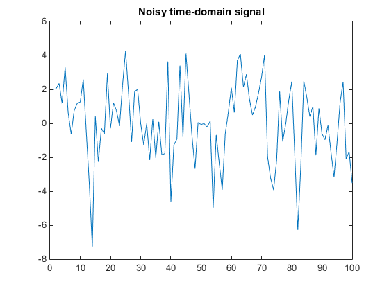
We add some random noise to the signal.

signal  = signal + 2 * randn( size( timeVec ), 'gpuArray' );
plot( signal(1:100) );
title( 'Noisy time-domain signal' );

Perform Spectral Analysis

Clearly, it is difficult to identify the frequency components from looking at this signal. We can see the frequency components by taking the discrete Fourier transform using the Fast Fourier Transform. Because we sent signal to the GPU, the FFT is performed on the GPU.

transformedSignal = fft( signal );

Compute the Power Spectral Density

The power spectral density measures the energy at various frequencies.

powerSpectrum = transformedSignal .* conj(transformedSignal) ./ numSamples;

Display the Power Spectral Density

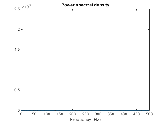
We can plot the powerSpectrum directly

frequencyVector = sampleFreq/2 * linspace( 0, 1, numSamples/2 + 1 );

plot( frequencyVector, real(powerSpectrum(1:numSamples/2+1)) );
title( 'Power spectral density' );
xlabel( 'Frequency (Hz)' );