Using GPU ARRAYFUN for Monte-Carlo Simulations
This example shows how prices for financial options can be calculated on a GPU using Monte-Carlo methods. Three simple types of exotic option are used as examples, but more complex options can be priced in a similar way.
This example is a function so that the helpers can be nested inside it.
function paralleldemo_gpu_optionpricing
This example uses long-running kernels, so cannot run if kernel execution on the GPU can time-out. A time-out is usually only active if the selected GPU is also driving a display.
dev = gpuDevice();
if dev.KernelExecutionTimeout
    error( 'pctexample:gpuoptionpricing:KernelTimeout', ...
        ['This example cannot run if kernel execution on the GPU can ', ...
        'time-out.'] );
end
Stock Price Evolution
We assume that prices evolve according to a log-normal distribution related to the risk-free interest rate, the dividend yield (if any), and the volatility in the market. All of these quantities are assumed fixed over the lifetime of the option. This gives the following stochastic differential equation for the price:
![$${\rm d}S = S \times
 \left[
 (r-d){\rm d}t + \sigma \epsilon \sqrt{{\rm d}t}
 \right]$$](../../examples/distcomp_product/paralleldemo_gpu_optionpricing_eq17284130511455291481.png)
where
 is the stock price,
 is the risk-free interest rate,
 is the stock's annual dividend yield,
 is the volatility of the price and
 represents a Gaussian white-noise process. Assuming that
 is log-normally distributed, this can be discretized to:
![$$S_{t+1} = S_{t} \times \exp{
 \left[
 \left(r - d - \frac{1}{2}\sigma^2\right)\Delta t
 + \sigma \epsilon \sqrt{ \Delta t }
 \right]
} $$](../../examples/distcomp_product/paralleldemo_gpu_optionpricing_eq14584843645873655464.png)
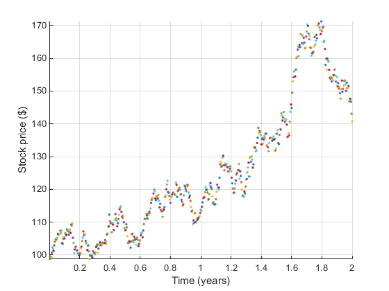
As an example let's use $100 of stock that yields a 1% dividend each year. The central government interest rate is assumed to be 0.5%. We examine a two-year time window sampled roughly daily. The market volatility is assumed to be 20% per annum.
stockPrice   = 100;   % Stock price starts at $100.
dividend     = 0.01;  % 1% annual dividend yield.
riskFreeRate = 0.005; % 0.5 percent.
timeToExpiry = 2;     % Lifetime of the option in years.
sampleRate   = 1/250; % Assume 250 working days per year.
volatility   = 0.20;  % 20% volatility.
We reset the random number generators to ensure repeatable results.
seed = 1234;
rng( seed );              % Reset the CPU random number generator.
parallel.gpu.rng( seed ); % Reset the GPU random number generator.
We can now loop over time to simulate the path of the stock price:
price = stockPrice;
time = 0;
hold on;
while time < timeToExpiry
    time = time + sampleRate;
    drift = (riskFreeRate - dividend - volatility*volatility/2)*sampleRate;
    perturbation = volatility*sqrt( sampleRate )*randn();
    price = price*exp(drift + perturbation);
    plot( time, price, '.' );
end
axis tight;
grid on;
xlabel( 'Time (years)' );
ylabel( 'Stock price ($)' );

Running on the GPU
To run stock price simulations on the GPU we first need to put the simulation loop inside a helper function:
    function finalStockPrice = simulateStockPrice(S,r,d,v,T,dT)
        t = 0;
        while t < T
            t = t + dT;
            dr = (r - d - v*v/2)*dT;
            pert = v*sqrt( dT )*randn();
            S = S*exp(dr + pert);
        end
        finalStockPrice = S;
    end
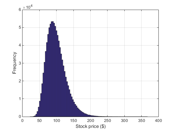
We can then call it thousands of times using arrayfun. To ensure the calculations happen on the GPU we make the input prices a GPU vector with one element per simulation. To accurately measure the calculation time on the GPU we use the gputimeit function.
% Create the input data.
N = 1000000;
startStockPrices = stockPrice*ones(N,1,'gpuArray');

% Run the simulations.
finalStockPrices = arrayfun( @simulateStockPrice, ...
    startStockPrices, riskFreeRate, dividend, volatility, ...
    timeToExpiry, sampleRate );
meanFinalPrice = mean(finalStockPrices);

% Measure the execution time of the function on the GPU using gputimeit.
% This requires us to store the |arrayfun| call in a function handle.
functionToTime = @() arrayfun(@simulateStockPrice, ...
    startStockPrices, riskFreeRate, dividend, volatility, ...
    timeToExpiry, sampleRate );
timeTaken = gputimeit(functionToTime);

fprintf( 'Calculated average price of $%1.4f in %1.3f secs.\n', ...
    meanFinalPrice, timeTaken );

clf;
hist( finalStockPrices, 100 );
xlabel( 'Stock price ($)' )
ylabel( 'Frequency' )
grid on;
Calculated average price of $98.9563 in 0.283 secs.

Pricing an Asian Option
As an example, let's use a European Asian Option based on the arithmetic mean of the price of the stock during the lifetime of the option. We can calculate the mean price by accumulating the price during the simulation. For a call option, the option is exercised if the average price is above the strike, and the payout is the difference between the two:
    function optionPrice = asianCallOption(S,r,d,v,x,T,dT)
        t = 0;
        cumulativePrice = 0;
        while t < T
            t = t + dT;
            dr = (r - d - v*v/2)*dT;
            pert = v*sqrt( dT )*randn();
            S = S*exp(dr + pert);
            cumulativePrice = cumulativePrice + S;
        end
        numSteps = (T/dT);
        meanPrice = cumulativePrice / numSteps;
        % Express the final price in today's money.
        optionPrice = exp(-r*T) * max(0, meanPrice - x);
    end
Again we use the GPU to run thousands of simulation paths using arrayfun. Each simulation path gives an independent estimate of the option price, and we therefore take the mean as our result.
strike = 95;   % Strike price for the option ($).

optionPrices = arrayfun( @asianCallOption, ...
    startStockPrices, riskFreeRate, dividend, volatility, strike, ...
    timeToExpiry, sampleRate );
meanOptionPrice = mean(optionPrices);

% Measure the execution time on the GPU and show the results.
functionToTime = @() arrayfun( @asianCallOption, ...
    startStockPrices, riskFreeRate, dividend, volatility, strike, ...
    timeToExpiry, sampleRate );
timeTaken = gputimeit(functionToTime);

fprintf( 'Calculated average price of $%1.4f in %1.3f secs.\n', ...
    meanOptionPrice, timeTaken );
Calculated average price of $8.7210 in 0.287 secs.
Pricing a Lookback Option
For this example we use a European-style lookback option whose payout is the difference between the minimum stock price and the final stock price over the lifetime of the option.
    function optionPrice = euroLookbackCallOption(S,r,d,v,T,dT)
        t = 0;
        minPrice = S;
        while t < T
            t = t + dT;
            dr = (r - d - v*v/2)*dT;
            pert = v*sqrt( dT )*randn();
            S = S*exp(dr + pert);
            if S<minPrice
                minPrice = S;
            end
        end
        % Express the final price in today's money.
        optionPrice = exp(-r*T) * max(0, S - minPrice);
    end
Note that in this case the strike price for the option is the minimum stock price. Because the final stock price is always greater than or equal to the minimum, the option is always exercised and is not really "optional".
optionPrices = arrayfun( @euroLookbackCallOption, ...
    startStockPrices, riskFreeRate, dividend, volatility, ...
    timeToExpiry, sampleRate );
meanOptionPrice = mean(optionPrices);

% Measure the execution time on the GPU and show the results.
functionToTime = @() arrayfun( @euroLookbackCallOption, ...
    startStockPrices, riskFreeRate, dividend, volatility, ...
    timeToExpiry, sampleRate );
timeTaken = gputimeit(functionToTime);

fprintf( 'Calculated average price of $%1.4f in %1.3f secs.\n', ...
    meanOptionPrice, timeTaken );
Calculated average price of $19.2711 in 0.286 secs.
Pricing a Barrier Option
This final example uses an "up and out" barrier option which becomes invalid if the stock price ever reaches the barrier level. If the stock price stays below the barrier level then the final stock price is used in a normal European call option calculation.
    function optionPrice = upAndOutCallOption(S,r,d,v,x,b,T,dT)
        t = 0;
        while (t < T) && (S < b)
            t = t + dT;
            dr = (r - d - v*v/2)*dT;
            pert = v*sqrt( dT )*randn();
            S = S*exp(dr + pert);
        end
        if S<b
            % Within barrier, so price as for a European option.
            optionPrice = exp(-r*T) * max(0, S - x);
        else
            % Hit the barrier, so the option is withdrawn.
            optionPrice = 0;
        end
    end
Note that we must now supply both a strike price for the option and the barrier price at which it becomes invalid:
strike  = 95;   % Strike price for the option ($).
barrier = 150;  % Barrier price for the option ($).

optionPrices = arrayfun( @upAndOutCallOption, ...
    startStockPrices, riskFreeRate, dividend, volatility, ...
    strike, barrier, ...
    timeToExpiry, sampleRate );
meanOptionPrice = mean(optionPrices);

% Measure the execution time on the GPU and show the results.
functionToTime = @() arrayfun( @upAndOutCallOption, ...
    startStockPrices, riskFreeRate, dividend, volatility, ...
    strike, barrier, ...
    timeToExpiry, sampleRate );
timeTaken = gputimeit(functionToTime);

fprintf( 'Calculated average price of $%1.4f in %1.3f secs.\n', ...
    meanOptionPrice, timeTaken );
Calculated average price of $6.8166 in 0.289 secs.
end