Large-Scale Bound Constrained Quadratic Programming

This example shows how to determine the shape of a circus tent by solving a large-scale quadratic optimization problem. The shape of a circus tent is determined by a constrained optimization problem. We will solve this problem with the function quadprog in Optimization Toolbox™.

The Problem
Lower Bound Constraint Surface
Initial Guess for Optimization
Resize Data for Optimization
Formulate Optimization Problem
Hessian Sparsity Structure
Run Optimization Solver
Reshape Solution Back to Original Size
Plot Circus Tent

The Problem

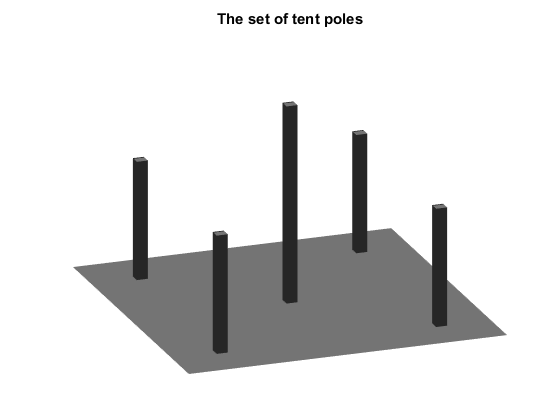
Imagine building a circus tent to cover a square lot. The tent has five poles that will be covered with an elastic material. From this structure, we want to find the natural shape of the tent. This natural shape corresponds to the minimum of a certain energy function computed from the surface position and squared norm of its gradient.

% Draw the tent poles.
largeL = zeros(36);
mask = [6 7 30 31];
largeL(mask,mask) = .3*ones(4);
largeL(18:19,18:19) = .5*ones(2);
xx = [1:5,5:6,6:15,15:16,16:25,25:26,26:30];
[XX,YY] = meshgrid(xx) ;
axis([1 30 1 30 0 .5],'off');
surface(XX,YY,largeL,'facecolor',[.5 .5 .5],'edgecolor','none');
light;
colormap(gray);
view([-20,30]);
title('The set of tent poles')

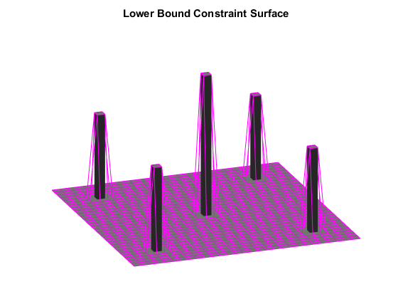
Lower Bound Constraint Surface

The supporting poles determine a lower bound for the tent, L. We can visualize the constraint by plotting it as a magenta mesh.

L = zeros(30);
E = ones(2);
L(15:16,15:16) = .5*E;
L(5:6,5:6) = .3*E;
L(25:26,5:6) = .3*E;
L(5:6,25:26) = .3*E;
L(25:26,25:26) = .3*E;

% Add L to the plot.
surface(L,'facecolor','none','edgecolor','m');
title('Lower Bound Constraint Surface')

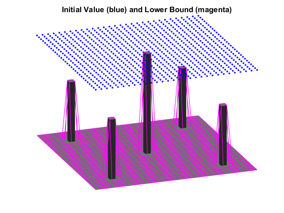
Initial Guess for Optimization

To solve this problem, we will find the height of the optimized surface at a finite number of points. Our initial guess, sstart, is shown in blue.

sstart = .5*ones(30,30);

% Add it to the plot.
surface(sstart,'FaceColor','none','LineStyle','none', ...
   'Marker','.','MarkerEdgeColor','blue')
title('Initial Value (blue) and Lower Bound (magenta)');
fig = gcf;
fig.Renderer = 'zbuffer';  % Markers do not show up in OpenGL.

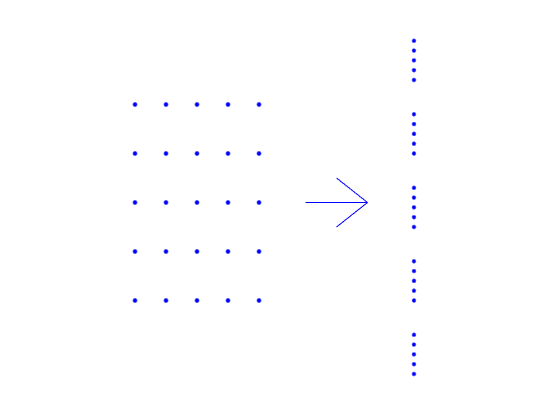
Resize Data for Optimization

In order to formulate the problem as a standard optimization problem, we resize both the matrices into vectors. L represents the initial values and sstart represents the lower boundary constraint.

low = reshape(L,900,1);
xstart = reshape(sstart,900,1);

% Illustrate the reordering.
% Draw grid points.
xx = 0:4;
[X, Y] = meshgrid(xx,xx);
gpts = plot(X(:),Y(:),'b.');
gpts.MarkerSize = 10;
axis off
axis([-2 12 -1.5 5.5])
hold on
% Draw arrow.
l(1) = line([7.5 6.5],[2 2.5]);
l(2) = line([7.5 6.5],[2 1.5]);
l(3) = line([7.5 5.5],[2 2]);
set(l,'color','b');
% Draw vector.
yy = 0.2*xx;
zz = [-1.5+yy,yy,1.5+yy,3+yy,4.5+yy];
vect = plot(9*ones(25,1),zz,'b.');
vect.MarkerSize = 9;
axis off;
hold off;

Formulate Optimization Problem

The surface formed by the elastic membrane is determined by the bound constrained optimization problem

   min{ c'*x+0.5*x'*H*x : low <= x }

where c'*x + 0.5*x'*H*x is the discrete approximation of the energy function. H and c are as follows:

H = delsq(numgrid('S',30+2));
h = 1/(30-1);
c = -h^2*ones(30^2,1);

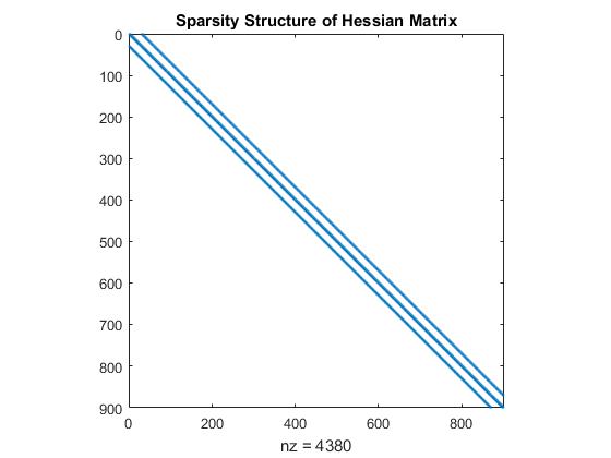
Hessian Sparsity Structure

Each point of the energy function is only affected by its immediate neighbors. Consequently the Hessian matrix H is sparse and has a special structure.

Because H is sparse we can use a large-scale algorithm to solve the optimization problem.

spy(H);
title('Sparsity Structure of Hessian Matrix');

Run Optimization Solver

The trust region reflective algorithm in quadprog solves bound constrained quadratic problems. We select this algorithm by setting an option with optimoptions. Then solve the problem by calling quadprog.

options = optimoptions('quadprog','Algorithm','trust-region-reflective',...
    'Display','off');
x = quadprog(H, c, [], [], [], [], low, [], xstart, options);

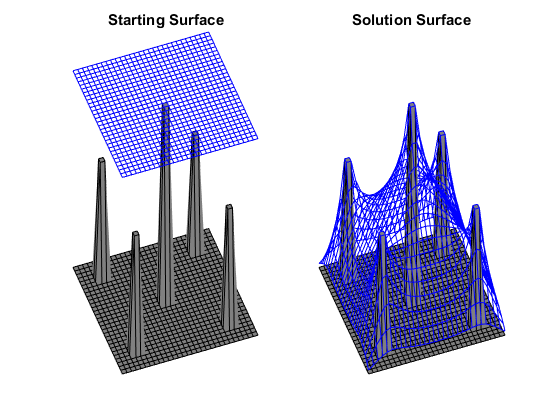
Reshape Solution Back to Original Size

Now obtain the surface solution by going back to the original ordering using reshape. Then plot this solution in blue mesh.

S = reshape(x,30,30);

% Plot the starting surface.
subplot(1,2,1);
surf(L,'facecolor',[.5 .5 .5]);
surface(sstart,'edgecolor','b','facecolor','none');
title('Starting Surface')
axis off
axis tight;
view([-20,30]);
% Plot the solution surface.
subplot(1,2,2);
surf(L,'facecolor',[.5 .5 .5]);
surface(S,'edgecolor','b','facecolor','none');
title('Solution Surface')
axis off
axis tight;
view([-20,30]);

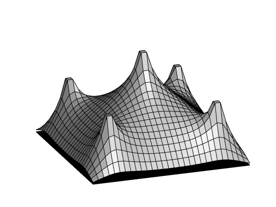
Plot Circus Tent

Let's now plot the solution that the optimization solver found.

subplot(1,1,1)
surf(L,'facecolor',[0 0 0]);
hold on;
surfl(S);
hold off;
axis tight;
axis off;
view([-20,30]);

Was this topic helpful?

Documentation