Documentation

This example shows how to recover a blurred image by solving a large-scale bound-constrained linear least-squares optimization problem.

The Problem

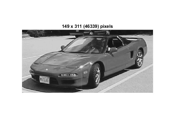
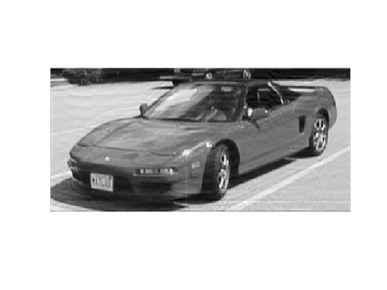
We will add motion blur to a photo of Mary Ann and Matthew sitting in Joe's car, then try to restore the original. Our starting image is this black and white image, contained the m x n matrix P. Each element in the matrix represents a pixel's gray intensity between black and white (0 and 1).

load optdeblur P
[m,n] = size(P);
mn = m*n;
imagesc(P);
colormap(gray);
axis off image;
title([int2str(m) ' x ' int2str(n) ' (' int2str(mn) ') pixels'])

Add Motion

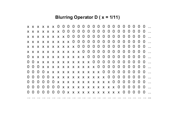
We can simulate the effect of vertical motion blurring by averaging each pixel with the 5 pixels above and below. We construct a sparse matrix D, that will do this with a single matrix multiply.

% Create D.
blur = 5;  mindex = 1:mn;  nindex = 1:mn;
for i = 1:blur
  mindex=[mindex i+1:mn 1:mn-i];
  nindex=[nindex 1:mn-i i+1:mn];
end
D = sparse(mindex,nindex,1/(2*blur+1));

% Draw a picture of D.
cla
axis off ij
xs = 25;
ys = 15;
xlim([0,xs+1]);
ylim([0,ys+1]);
[ix,iy] = meshgrid(1:(xs-1),1:(ys-1));
l = abs(ix-iy)<=5;
text(ix(l),iy(l),'x')
text(ix(~l),iy(~l),'0')
text(xs*ones(ys,1),1:ys,'...');
text(1:xs,ys*ones(xs,1),'...');
title('Blurring Operator D ( x = 1/11)')

Apply Blurring Operator

We multiply the image by this operator to create the blurred image. P is the original image, D is the operator, and G is the blurred image.

G = D*P(:);
imagesc(reshape(G,m,n));
axis off image;

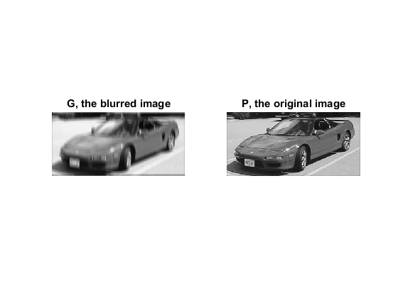
The Blurred Image

Now, let's pretend Joe took this blurred picture G from a moving elevator. Assume we know how fast the elevator is moving, so we know the blurring operator D. How well can we remove the blur and recover the original image P?

The simplest approach is to solve the least squares problem:

  min( || D*P(:) - G||^2 )

subplot(1,2,1);
imagesc(reshape(G(:),m,n)); axis off image;
title('G, the blurred image');
subplot(1,2,2);
imagesc(reshape(P(:),m,n)); axis off image;
title('P, the original image');

Regularization Term

In practice the results obtained with this simple approach tend to be noisy. To compensate for this, a regularization term is added:

     0.0004*|| L*P ||^2

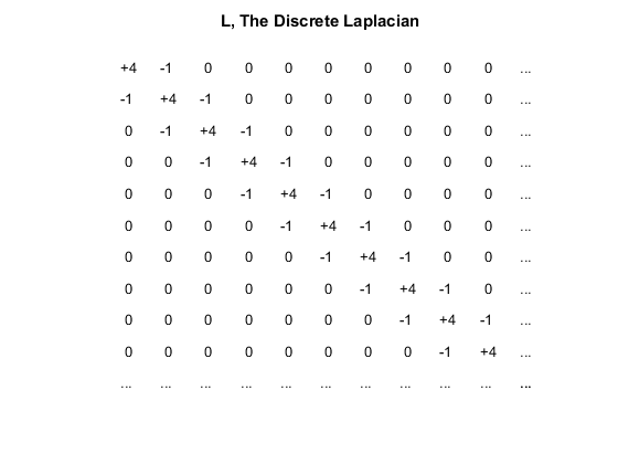
L is the discrete Laplacian, which relates each pixel to those surrounding it. Since we know we are looking for a gray intensity, we also impose the constraint that the elements of P must fall between 0 and 1.

% Create L.
L = sparse( [1:mn,2:mn,1:mn-1],  [1:mn,1:mn-1,2:mn], ...
   [4*ones(1,mn) -1*ones(1,2*(mn-1))]  );

% Draw a picture of L.
subplot(1,1,1) ;
delete(gca);
axis ij
axis off;
xs=11;
ys=11;
xlim([0,xs+1]);
ylim([0,ys+1]);
[ix,iy]=meshgrid(1:(xs-1),1:(ys-1));
four=(ix==iy);
one=(abs(ix-iy)==1);
text(ix(one),iy(one),'-1')
text(ix(four),iy(four),'+4')
text(ix(~four & ~one),iy(~four & ~one),' 0')
text(xs*ones(ys,1),1:ys,'...');
text(1:xs,ys*ones(xs,1),'...');
title('L, The Discrete Laplacian')

Set Up Problem to Deblur Image

To obtain the deblurred picture we want to solve for P:

  min( || D*P(:) - G(:) ||^2 + 0.0004*|| L*P(:) ||^2 )

We can simplify this expression by defining A and b:

  A = [D ; 0.02*L]; b = [ G(:) ; zeros(mn,1) ];

which changes the last equation to:

  min( || A*P(:) - b ||^2 )

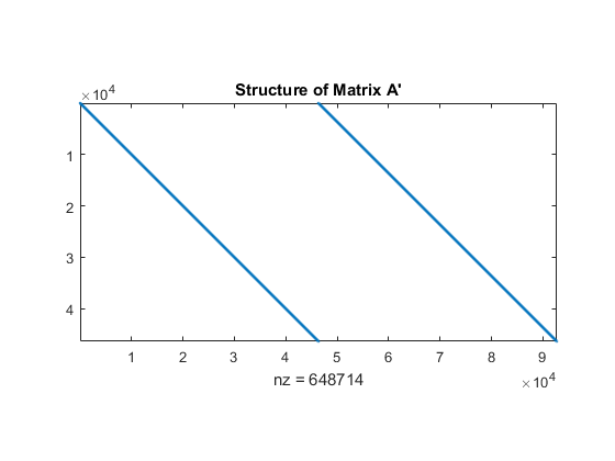
subject to 0<=P<=1. Both matrices D and L relate each pixel to a few of its neighbors. This makes A structured and sparse.

A = [D ; 0.02*L]; b = [ G(:) ; zeros(mn,1) ];
spy(A');
axis equal tight
title('Structure of Matrix A''');

Solve Optimization Problem

Because A is sparse, we can use a large-scale algorithm to solve this linear least squares optimization problem. We call LSQLIN with A, b, lower bounds, upper bounds, and options.

options = optimoptions('lsqlin','Algorithm','trust-region-reflective',...
    'Display','off');
x = lsqlin(A, b, [], [], [], [], zeros(mn,1), ones(mn,1), [], options);
imagesc(reshape(x,m,n))
axis off image

Compare Images

Let's compare the blurred and deblurred pictures.

subplot(1,2,1);
imagesc(reshape(G,m,n)); axis image; axis off;
title('Blurred');

subplot(1,2,2);
imagesc(reshape(x,m,n)); axis image; axis off;
title('De-Blurred');