Maximize Long-Term Investments Using Linear Programming
This example shows how to use the linprog solver in Optimization Toolbox® to solve an investment problem with deterministic returns over a fixed number of years T. The problem is to allocate your money over available investments to maximize your final wealth.
Problem Formulation
Suppose that you have an initial amount of money Capital_0 to invest over a time period of T years in N zero-coupon bonds. Each bond pays an interest rate that compounds each year, and pays the principal plus compounded interest at the end of a maturity period. The objective is to maximize the total amount of money after T years.
You can include a constraint that no single investment is more than a certain fraction of your total capital.
This example shows the problem setup on a small case first, and then formulates the general case.
You can model this as a linear programming problem. Therefore, to optimize your wealth, formulate the problem for solution by the linprog solver.
Introductory Example
Start with a small example:
The starting amount to invest
Capital_0is $1000.The time period
Tis 5 years.The number of bonds
Nis 4.To model uninvested money, have one option B0 available every year that has a maturity period of 1 year and a interest rate of 0%.
Bond 1, denoted by B1, can be purchased in year 1, has a maturity period of 4 years, and interest rate of 2%.
Bond 2, denoted by B2, can be purchased in year 5, has a maturity period of 1 year, and interest rate of 4%.
Bond 3, denoted by B3, can be purchased in year 2, has a maturity period of 4 years, and interest rate of 6%.
Bond 4, denoted by B4, can be purchased in year 2, has a maturity period of 3 years, and interest rate of 6%.
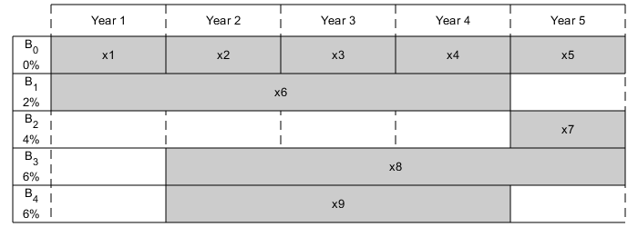
By splitting up the first option B0 into 5 bonds with maturity period of 1 year and interest rate of 0%, this problem can be equivalently modeled as having a total of 9 available bonds, such that for k=1..9
Entry
kof vectorPurchaseYearsrepresents the year that bondkis available for purchase.Entry
kof vectorMaturityrepresents the maturity period of bond
 k.Entry
kof vectorInterestRatesrepresents the interest rate of bond
 k.
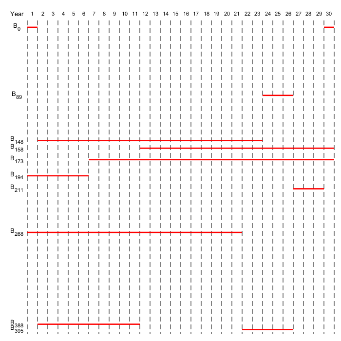
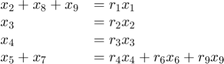
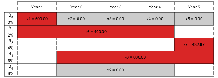
Visualize this problem by horizontal bars that represent the available purchase times and durations for each bond.
% Time period in years
T = 5;
% Number of bonds
N = 4;
% Initial amount of money
Capital_0 = 1000;
% Total number of buying oportunities
nPtotal = N+T;
% Purchase times
PurchaseYears = [1;2;3;4;5;1;5;2;2];
% Bond durations
Maturity = [1;1;1;1;1;4;1;4;3];
% Interest rates
InterestRates = [0;0;0;0;0;2;4;6;6];

plotInvestments(N,PurchaseYears,Maturity,InterestRates)
Decision Variables
Represent your decision variables by a vector x, where x(k) is the dollar amount of investment in bond k, for k=1..9. Upon maturity, the payout for investment x(k) is
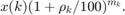
Define
 as the total return of bond
 k:
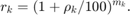
% Total returns
finalReturns = (1+InterestRates/100).^Maturity;
Objective Function
The goal is to choose investments to maximize the amount of money collected at the end of year T. From the plot, you see that investments are collected at various intermediate years and reinvested. At the end of year T, the money returned from investments 5, 7, and 8 can be collected and represents your final wealth:
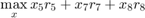
To place this problem into the form linprog solves, turn this maximization problem into a minimization problem using the negative of the coefficients of x(j):

with
![$$ f = [0; 0; 0; 0; -r_5; 0; -r_7;-r_8; 0] $$](../../examples/optim_product/LongTermInvestmentsExample_eq13060452493453761734.png)
f = zeros(nPtotal,1);
f([5,7,8]) = [-finalReturns(5),-finalReturns(7),-finalReturns(8)];
Linear Constraints: Invest No More Than You Have
Every year, you have a certain amount of money available to purchase bonds. Starting with year 1, you can invest the initial capital in the purchase options
 and
and
 , so:
, so:
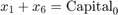
Then for the following years, you collect the returns from maturing bonds, and reinvest them in new available bonds to obtain the system of equations:
Write these equations in the form
 , where each row of the
 matrix corresponds to the equality that needs to be satisfied that year:
![$$Aeq = \left[ \begin{array}{ccccccccc}
1 & 0 & 0 & 0 & 0 & 1 & 0 & 0 & 0\\
-r_1 & 1 & 0 & 0 & 0 & 0 & 0 & 1 & 1\\
0 & -r_2 & 1 & 0 & 0 & 0 & 0 & 0 & 0\\
0 & 0 & -r_3 & 1 & 0 & 0 & 0 & 0 & 0\\
0 & 0 & 0 & -r_4 & 1 & -r_6 & 1 & 0 & -r_9 \end{array}
\right] $$](../../examples/optim_product/LongTermInvestmentsExample_eq08538447291580604117.png)
![$$ beq = \left[ \begin{array}{c} \mathrm{Capital}_0 \\ 0 \\ 0 \\ 0 \end{array} \right] $$](../../examples/optim_product/LongTermInvestmentsExample_eq11310712372127110506.png)
Aeq = spalloc(N+1,nPtotal,15);
Aeq(1,[1,6]) = 1;
Aeq(2,[1,2,8,9]) = [-1,1,1,1];
Aeq(3,[2,3]) = [-1,1];
Aeq(4,[3,4]) = [-1,1];
Aeq(5,[4:7,9]) = [-finalReturns(4),1,-finalReturns(6),1,-finalReturns(9)];

beq = zeros(T,1);
beq(1) = Capital_0;
Bound Constraints: No Borrowing
Because each amount invested must be positive, each entry in the solution vector
 must be positive. Include this constraint by setting a lower bound
 lb on the solution vector
. There is no explicit upper bound on the solution vector. Thus, set the upper bound ub to empty.
lb = zeros(size(f));
ub = [];
Solve the Problem
Solve this problem with no constraints on the amount you can invest in a bond. The interior-point algorithm can be used to solve this type of linear programming problem.
options = optimoptions('linprog','Algorithm','interior-point');
[xsol,fval,exitflag] = linprog(f,[],[],Aeq,beq,lb,ub,[],options);
Solution found during presolve.
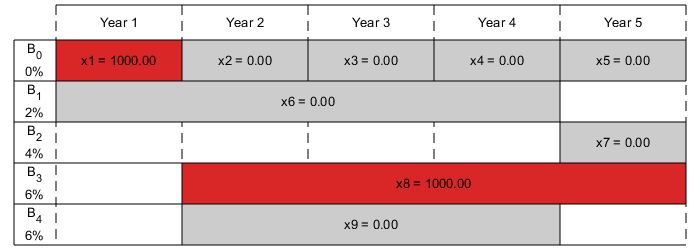
Visualize the Solution
The exit flag is 1, indicating that the solver found a solution. The value -fval, returned as the second linprog output argument, corresponds to the final wealth. Plot your investments over time.
fprintf('After %d years, the return for the initial $%g is $%g \n',...
    T,Capital_0,-fval);

plotInvestments(N,PurchaseYears,Maturity,InterestRates,xsol)
After 5 years, the return for the initial $1000 is $1262.48
Optimal Investment with Limited Holdings
To diversify your investments, you can choose to limit the amount invested in any one bond to a certain percentage Pmax of the total capital that year (including the returns for bonds that are currently in their maturity period). You obtain the following system of inequalities:
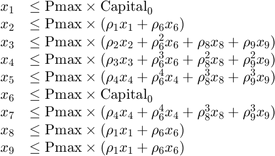
Place these inequalities in the matrix form Ax <= b.
To set up the system of inequalities, first generate a matrix yearlyReturns that contains the return for the bond indexed by i at year j in row i and column j. Represent this system as a sparse matrix.
% Maximum percentage to invest in any bond
Pmax = 0.6;

% Build the return for each bond over the maturity period as a sparse
% matrix
cumMaturity = [0;cumsum(Maturity)];
xr = zeros(cumMaturity(end-1),1);
yr = zeros(cumMaturity(end-1),1);
cr = zeros(cumMaturity(end-1),1);
for i = 1:nPtotal
    mi = Maturity(i); % maturity of bond i
    pi = PurchaseYears(i); % purchase year of bond i
    idx = cumMaturity(i)+1:cumMaturity(i+1); % index into xr, yr and cr
    xr(idx) = i; % bond index
    yr(idx) = pi+1:pi+mi; % maturing years
    cr(idx) = (1+InterestRates(i)/100).^(1:mi); % returns over the maturity period
end
yearlyReturns = sparse(xr,yr,cr,nPtotal,T+1);

% Build the system of inequality constraints
A = -Pmax*yearlyReturns(:,PurchaseYears)'+ speye(nPtotal);

% Left-hand side
b = zeros(nPtotal,1);
b(PurchaseYears == 1) = Pmax*Capital_0;
Solve the problem by investing no more than 60% in any one asset. Plot the resulting purchases. Notice that your final wealth is less than the investment without this constraint.
[xsol,fval,exitflag] = linprog(f,A,b,Aeq,beq,lb,ub,[],options);

fprintf('After %d years, the return for the initial $%g is $%g \n',...
    T,Capital_0,-fval);

plotInvestments(N,PurchaseYears,Maturity,InterestRates,xsol)
Minimum found that satisfies the constraints.

Optimization completed because the objective function is non-decreasing in
feasible directions, to within the selected value of the function tolerance,
and constraints are satisfied to within the selected value of the constraint
tolerance.

After 5 years, the return for the initial $1000 is $1207.78
Model of Arbitrary Size
Create a model for a general version of the problem. Illustrate it using T = 30 years and 400 randomly generated bonds with interest rates from 1 to 6%. This setup results in a linear programming problem with 430 decision variables. The system of equality constraints is represented by a sparse matrix Aeq of dimension 30-by-430 and the system of inequalities is represented by a sparse matrix A of dimension 430-by-430.
% for reproducibility
rng default
% Initial amount of money
Capital_0 = 1000;
% Time period in years
T = 30;
% Number of bonds
N = 400;
% Total number of buying oportunities
nPtotal = N+T;
% Generate random maturity durations
Maturity = randi([1 T-1],nPtotal,1);
% Bond 1 has a maturity period of 1 year
Maturity(1:T) = 1;
% Generate random yearly interest rate for each bond
InterestRates = randi(6,nPtotal,1);
% Bond 1 has an interest rate of 0 (not invested)
InterestRates(1:T) = 0;
% Compute the return at the end of the maturity period for each bond:
finalReturns = (1+InterestRates/100).^Maturity;

% Generate random purchase years for each option
PurchaseYears = zeros(nPtotal,1);
% Bond 1 is available for purchase every year
PurchaseYears(1:T)=1:T;
for i=1:N
    % Generate a random year for the bond to mature before the end of
    % the T year period
    PurchaseYears(i+T) = randi([1 T-Maturity(i+T)+1]);
end

% Compute the years where each bond reaches maturity
SaleYears = PurchaseYears + Maturity;

% Initialize f to 0
f = zeros(nPtotal,1);
% Indices of the sale oportunities at the end of year T
SalesTidx = SaleYears==T+1;
% Expected return for the sale oportunities at the end of year T
ReturnsT = finalReturns(SalesTidx);
% Objective function
f(SalesTidx) = -ReturnsT;


% Generate the system of equality constraints.
% For each purchase option, put a coefficient of 1 in the row corresponding
% to the year for the purchase option and the column corresponding to the
% index of the purchase oportunity
xeq1 = PurchaseYears;
yeq1 = (1:nPtotal)';
ceq1 = ones(nPtotal,1);

% For each sale option, put -\rho_k, where \rho_k is the interest rate for the
% associated bond that is being sold, in the row corresponding to the
% year for the sale option and the column corresponding to the purchase
% oportunity
xeq2 = SaleYears(~SalesTidx);
yeq2 = find(~SalesTidx);
ceq2 = -finalReturns(~SalesTidx);

% Generate the sparse equality matrix
Aeq = sparse([xeq1; xeq2], [yeq1; yeq2], [ceq1; ceq2], T, nPtotal);

% Generate the right-hand side
beq = zeros(T,1);
beq(1) = Capital_0;

% Build the system of inequality constraints
% Maximum percentage to invest in any bond
Pmax = 0.4;

% Build the returns for each bond over the maturity period
cumMaturity = [0;cumsum(Maturity)];
xr = zeros(cumMaturity(end-1),1);
yr = zeros(cumMaturity(end-1),1);
cr = zeros(cumMaturity(end-1),1);
for i = 1:nPtotal
    mi = Maturity(i); % maturity of bond i
    pi = PurchaseYears(i); % purchase year of bond i
    idx = cumMaturity(i)+1:cumMaturity(i+1); % index into xr, yr and cr
    xr(idx) = i; % bond index
    yr(idx) = pi+1:pi+mi; % maturing years
    cr(idx) = (1+InterestRates(i)/100).^(1:mi); % returns over the maturity period
end
yearlyReturns = sparse(xr,yr,cr,nPtotal,T+1);

% Build the system of inequality constraints
A = -Pmax*yearlyReturns(:,PurchaseYears)'+ speye(nPtotal);

% Left-hand side
b = zeros(nPtotal,1);
b(PurchaseYears==1) = Pmax*Capital_0;

% Add the lower-bound constraints to the problem.
lb = zeros(nPtotal,1);
Solution with No Holding Limit
First, solve the linear programming problem without inequality constraints using the interior-point algorithm.
% Solve the problem without inequality constraints
options = optimoptions('linprog','Algorithm','interior-point');
tic
[xsol,fval,exitflag] = linprog(f,[],[],Aeq,beq,lb,[],[],options);
toc

fprintf('\nAfter %d years, the return for the initial $%g is $%g \n',...
    T,Capital_0,-fval);
Minimum found that satisfies the constraints.

Optimization completed because the objective function is non-decreasing in
feasible directions, to within the selected value of the function tolerance,
and constraints are satisfied to within the selected value of the constraint
tolerance.

Elapsed time is 0.017012 seconds.

After 30 years, the return for the initial $1000 is $5167.58
Solution with Limited Holdings
Now, solve the problem with the inequality constraints.
% Solve the problem with inequality constraints
options = optimoptions('linprog','Algorithm','interior-point');
tic
[xsol,fval,exitflag] = linprog(f,A,b,Aeq,beq,lb,[],[],options);
toc

fprintf('\nAfter %d years, the return for the initial $%g is $%g \n',...
    T,Capital_0,-fval);
Minimum found that satisfies the constraints.

Optimization completed because the objective function is non-decreasing in
feasible directions, to within the selected value of the function tolerance,
and constraints are satisfied to within the selected value of the constraint
tolerance.

Elapsed time is 1.552141 seconds.

After 30 years, the return for the initial $1000 is $5095.26
Even though the number of constraints increased by an order of 10, the time for the solver to find a solution increased by an order of 100. This performance discrepancy is partially caused by dense columns in the inequality system shown in matrix A. These columns correspond to bonds with a long maturity period, as shown in the following graph.
% Number of nonzero elements per column
nnzCol = sum(spones(A));

% Plot the maturity length vs. the number of nonzero elements for each bond
figure;
plot(Maturity,nnzCol,'o');
xlabel('Maturity period of bond k')
ylabel('Number of nonzero in column k of A')
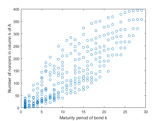
Dense columns in the constraints lead to dense blocks in the solver's internal matrices, yielding a loss of efficiency of its sparse methods. To speed up the solver, try the dual-simplex algorithm, which is less sensitive to column density.
% Solve the problem with inequality constraints using dual simplex
options = optimoptions('linprog','Algorithm','dual-simplex');
tic
[xsol,fval,exitflag] = linprog(f,A,b,Aeq,beq,lb,[],[],options);
toc

fprintf('\nAfter %d years, the return for the initial $%g is $%g \n',...
    T,Capital_0,-fval);
Optimal solution found.

Elapsed time is 0.224239 seconds.

After 30 years, the return for the initial $1000 is $5095.26
In this case, the dual-simplex algorithm took much less time to obtain the same solution.
Qualitative Result Analysis
To get a feel for the solution found by linprog, compare it to the amount fmax that you would get if you could invest all of your starting money in one bond with a 6% interest rate (the maximum interest rate) over the full 30 year period. You can also compute the equivalent interest rate corresponding to your final wealth.
% Maximum amount
fmax = Capital_0*(1+6/100)^T;
% Ratio (in percent)
rat = -fval/fmax*100;
% Equivalent interest rate (in percent)
rsol = ((-fval/Capital_0)^(1/T)-1)*100;

fprintf(['The amount collected is %g%% of the maximum amount $%g '...
    'that you would obtain from investing in one bond.\n'...
    'Your final wealth corresponds to a %g%% interest rate over the %d year '...
    'period.\n'], rat, fmax, rsol, T)

plotInvestments(N,PurchaseYears,Maturity,InterestRates,xsol,false)
The amount collected is 88.7137% of the maximum amount $5743.49 that you would obtain from investing in one bond.
Your final wealth corresponds to a 5.57771% interest rate over the 30 year period.