Minimax Optimization
This example shows how to solve a nonlinear filter design problem using a minimax optimization algorithm, fminimax, in Optimization Toolbox™. Note that to run this example you must have the Signal Processing Toolbox™ installed.
Set Finite Precision Parameters
Consider an example for the design of finite precision filters. For this, you need to specify not only the filter design parameters such as the cut-off frequency and number of coefficients, but also how many bits are available since the design is in finite precision.
nbits  = 8;         % How many bits have we to realize filter
maxbin = 2^nbits-1; % Maximum number expressable in nbits bits
n      = 4;         % Number of coefficients (order of filter plus 1)
Wn     = 0.2;       % Cutoff frequency for filter
Rp     = 1.5;       % Decibels of ripple in the passband
w      = 128;       % Number of frequency points to take
Continuous Design First
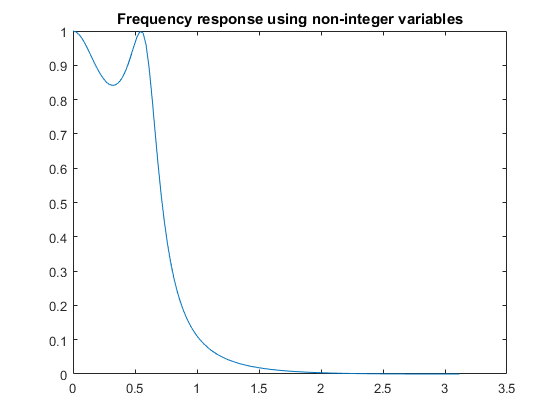
This is a continuous filter design; we use cheby1, but we could also use ellip, yulewalk or remez here:
[b1,a1] = cheby1(n-1,Rp,Wn);

[h,w] = freqz(b1,a1,w); % Frequency response
h = abs(h);             % Magnitude response
plot(w, h)
title('Frequency response using non-integer variables')
x = [b1,a1];            % The design variables
Set Bounds for Filter Coefficients
We now set bounds on the maximum and minimum values:
if (any(x < 0))
%   If there are negative coefficients - must save room to use a sign bit
%   and therefore reduce maxbin
    maxbin = floor(maxbin/2);
    vlb = -maxbin * ones(1, 2*n)-1;
    vub = maxbin * ones(1, 2*n);
else
%   otherwise, all positive
    vlb = zeros(1,2*n);
    vub = maxbin * ones(1, 2*n);
end
Scale Coefficients
Set the biggest value equal to maxbin and scale other filter coefficients appropriately.
[m, mix] = max(abs(x));
factor =  maxbin/m;
x =  factor * x;    % Rescale other filter coefficients
xorig = x;

xmask = 1:2*n;
% Remove the biggest value and the element that controls D.C. Gain
% from the list of values that can be changed.
xmask(mix) = [];
nx = 2*n;
Set Optimization Criteria
Using optimoptions, adjust the termination criteria to reasonably high values to promote short running times. Also turn on the display of results at each iteration:
options = optimoptions('fminimax','TolX',0.1,'TolFun',1e-4,...
    'TolCon',1e-6,'Display','iter');
Minimize the Absolute Maximum Values
We need to minimize absolute maximum values, so we set options.MinAbsMax to the number of frequency points:
if length(w) == 1
   options = optimoptions(options,'MinAbsMax',w);
else
   options = optimoptions(options,'MinAbsMax',length(w));
end
Eliminate First Value for Optimization
Discretize and eliminate first value and perform optimization by calling FMINIMAX:
[x, xmask] = elimone(x, xmask, h, w, n, maxbin)

niters = length(xmask);
disp(sprintf('Performing %g stages of optimization.\n\n', niters));

for m = 1:niters
    fun = @(xfree)filtobj(xfree,x,xmask,n,h,maxbin); % objective
    confun = @(xfree)filtcon(xfree,x,xmask,n,h,maxbin); % nonlinear constraint
    disp(sprintf('Stage: %g \n', m));
    x(xmask) = fminimax(fun,x(xmask),[],[],[],[],vlb(xmask),vub(xmask),...
        confun,options);
    [x, xmask] = elimone(x, xmask, h, w, n, maxbin);
end
x =

  Columns 1 through 7

    0.5441    1.6323    1.6323    0.5441   57.1653 -127.0000  108.0000

  Column 8

  -33.8267


xmask =

     1     2     3     4     5     8

Performing 6 stages of optimization.


Stage: 1


                  Objective        Max     Line search     Directional
 Iter F-count         value    constraint   steplength      derivative   Procedure
    0      8              0    0.00329174
    1     17      0.0001845      3.34e-07            1          0.0143

Local minimum possible. Constraints satisfied.

fminimax stopped because the size of the current search direction is less than
twice the selected value of the step size tolerance and constraints are
satisfied to within the selected value of the constraint tolerance.


Stage: 2


                  Objective        Max     Line search     Directional
 Iter F-count         value    constraint   steplength      derivative   Procedure
    0      7              0     0.0414182
    1     15        0.01649     0.0002558            1           0.261
    2     23        0.01544     6.124e-07            1         -0.0282    Hessian modified

Local minimum possible. Constraints satisfied.

fminimax stopped because the size of the current search direction is less than
twice the selected value of the step size tolerance and constraints are
satisfied to within the selected value of the constraint tolerance.


Stage: 3


                  Objective        Max     Line search     Directional
 Iter F-count         value    constraint   steplength      derivative   Procedure
    0      6              0     0.0716961
    1     13        0.05943     6.763e-11            1           0.776

Local minimum possible. Constraints satisfied.

fminimax stopped because the size of the current search direction is less than
twice the selected value of the step size tolerance and constraints are
satisfied to within the selected value of the constraint tolerance.


Stage: 4


                  Objective        Max     Line search     Directional
 Iter F-count         value    constraint   steplength      derivative   Procedure
    0      5              0      0.129938
    1     11        0.04278      4.23e-11            1           0.183

Local minimum possible. Constraints satisfied.

fminimax stopped because the size of the current search direction is less than
twice the selected value of the step size tolerance and constraints are
satisfied to within the selected value of the constraint tolerance.


Stage: 5


                  Objective        Max     Line search     Directional
 Iter F-count         value    constraint   steplength      derivative   Procedure
    0      4              0     0.0901749
    1      9        0.03867    -1.562e-10            1           0.256

Local minimum possible. Constraints satisfied.

fminimax stopped because the size of the current search direction is less than
twice the selected value of the step size tolerance and constraints are
satisfied to within the selected value of the constraint tolerance.


Stage: 6


                  Objective        Max     Line search     Directional
 Iter F-count         value    constraint   steplength      derivative   Procedure
    0      3              0       0.11283
    1      7        0.05033     9.714e-17            1           0.197

Local minimum possible. Constraints satisfied.

fminimax stopped because the size of the current search direction is less than
twice the selected value of the step size tolerance and constraints are
satisfied to within the selected value of the constraint tolerance.
Check Nearest Integer Values
See if nearby values produce a for better filter.
xold = x;
xmask = 1:2*n;
xmask([n+1, mix]) = [];
x = x + 0.5;
for i = xmask
    [x, xmask] = elimone(x, xmask, h, w, n, maxbin);
end
xmask = 1:2*n;
xmask([n+1, mix]) = [];
x = x - 0.5;
for i = xmask
    [x, xmask] = elimone(x, xmask, h, w, n, maxbin);
end
if any(abs(x) > maxbin)
  x = xold;
end
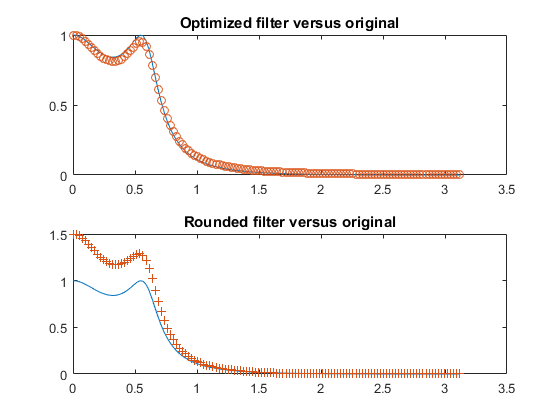
Frequency Response Comparisons
We first plot the frequency response of the filter and we compare it to a filter where the coefficients are just rounded up or down:
subplot(211)
bo = x(1:n);
ao = x(n+1:2*n);
h2 = abs(freqz(bo,ao,128));
plot(w,h,w,h2,'o')
title('Optimized filter versus original')

xround = round(xorig)
b = xround(1:n);
a = xround(n+1:2*n);
h3 = abs(freqz(b,a,128));
subplot(212)
plot(w,h,w,h3,'+')
title('Rounded filter versus original')
fig = gcf;
fig.NextPlot = 'replace';
xround =

     1     2     2     1    57  -127   108   -34