Minimizing an Expensive Optimization Problem Using Parallel Computing Toolbox™
This example shows how to how to speed up the minimization of an expensive optimization problem using functions in Optimization Toolbox™ and Global Optimization Toolbox. In the first part of the example we solve the optimization problem by evaluating functions in a serial fashion and in the second part of the example we solve the same problem using the parallel for loop (parfor) feature by evaluating functions in parallel. We compare the time taken by the optimization function in both cases.
Expensive Optimization Problem
For the purpose of this example, we solve a problem in four variables, where the objective and constraint functions are made artificially expensive by pausing.
type expensive_objfun.m
type expensive_confun.m
function f = expensive_objfun(x)
%EXPENSIVE_OBJFUN An expensive objective function used in optimparfor example.

%   Copyright 2007-2014 The MathWorks, Inc.
%   $Revision: 1.1.8.2 $  $Date: 2013/05/04 00:47:14 $

% Simulate an expensive function by pausing
pause(0.1)
% Evaluate objective function
f = exp(x(1)) * (4*x(3)^2 + 2*x(4)^2 + 4*x(1)*x(2) + 2*x(2) + 1);

function [c,ceq] = expensive_confun(x)
%EXPENSIVE_CONFUN An expensive constraint function used in optimparfor example.

%   Copyright 2007-2014 The MathWorks, Inc.
%   $Revision: 1.1.8.2 $  $Date: 2013/05/04 00:47:13 $

% Simulate an expensive function by pausing
pause(0.1);
% Evaluate constraints
c = [1.5 + x(1)*x(2)*x(3) - x(1) - x(2) - x(4);
     -x(1)*x(2) + x(4) - 10];
% No nonlinear equality constraints:
ceq = [];
Minimizing Using fmincon
We are interested in measuring the time taken by fmincon in serial so that we can compare it to the parallel fmincon evaluation.
startPoint = [-1 1 1 -1];
options = optimoptions('fmincon','Display','iter','Algorithm','sqp');
startTime = tic;
xsol = fmincon(@expensive_objfun,startPoint,[],[],[],[],[],[],@expensive_confun,options);
time_fmincon_sequential = toc(startTime);
fprintf('Serial FMINCON optimization takes %g seconds.\n',time_fmincon_sequential);
                                                          Norm of First-order
 Iter F-count            f(x) Feasibility  Steplength        step  optimality
    0       5    1.839397e+00   1.500e+00                           3.311e+00
    1      12   -8.841073e-01   4.019e+00   4.900e-01   2.335e+00   7.015e-01
    2      17   -1.382832e+00   0.000e+00   1.000e+00   1.142e+00   9.272e-01
    3      22   -2.241952e+00   0.000e+00   1.000e+00   2.447e+00   1.481e+00
    4      27   -3.145762e+00   0.000e+00   1.000e+00   1.756e+00   5.464e+00
    5      32   -5.277523e+00   6.413e+00   1.000e+00   2.224e+00   1.357e+00
    6      37   -6.310709e+00   0.000e+00   1.000e+00   1.099e+00   1.309e+00
    7      43   -6.447956e+00   0.000e+00   7.000e-01   2.191e+00   3.631e+00
    8      48   -7.135133e+00   0.000e+00   1.000e+00   3.719e-01   1.205e-01
    9      53   -7.162732e+00   0.000e+00   1.000e+00   4.083e-01   2.935e-01
   10      58   -7.178390e+00   0.000e+00   1.000e+00   1.591e-01   3.110e-02
   11      63   -7.180399e+00   1.191e-05   1.000e+00   2.644e-02   1.553e-02
   12      68   -7.180408e+00   0.000e+00   1.000e+00   1.140e-02   5.584e-03
   13      73   -7.180411e+00   0.000e+00   1.000e+00   1.764e-03   4.677e-04
   14      78   -7.180412e+00   0.000e+00   1.000e+00   8.827e-05   1.304e-05
   15      83   -7.180412e+00   0.000e+00   1.000e+00   1.528e-06   1.023e-07

Local minimum found that satisfies the constraints.

Optimization completed because the objective function is non-decreasing in
feasible directions, to within the default value of the function tolerance,
and constraints are satisfied to within the default value of the constraint tolerance.


Serial FMINCON optimization takes 18.1397 seconds.
Minimizing Using Genetic Algorithm
Since ga usually takes many more function evaluations than fmincon, we remove the expensive constraint from this problem and perform unconstrained optimization instead; we pass empty ([]) for constraints. In addition, we limit the maximum number of generations to 15 for ga so that ga can terminate in a reasonable amount of time. We are interested in measuring the time taken by ga so that we can compare it to the parallel ga evaluation. Note that running ga requires Global Optimization Toolbox.
rng default % for reproducibility
try
    gaAvailable = false;
    nvar = 4;
    gaoptions = gaoptimset('Generations',15,'Display','iter');
    startTime = tic;
    gasol = ga(@expensive_objfun,nvar,[],[],[],[],[],[],[],gaoptions);
    time_ga_sequential = toc(startTime);
    fprintf('Serial GA optimization takes %g seconds.\n',time_ga_sequential);
    gaAvailable = true;
catch ME
    warning(message('optimdemos:optimparfor:gaNotFound'));
end
                               Best           Mean      Stall
Generation      f-count        f(x)           f(x)    Generations
    1           100      -6.433e+16      -1.287e+15        0
    2           150      -1.501e+17      -7.138e+15        0
    3           200      -7.878e+26      -1.576e+25        0
    4           250      -8.664e+27      -1.466e+26        0
    5           300      -1.096e+28      -2.062e+26        0
    6           350      -5.422e+33      -1.145e+32        0
    7           400      -1.636e+36      -3.316e+34        0
    8           450      -2.933e+36      -1.513e+35        0
    9           500      -1.351e+40      -2.705e+38        0
   10           550      -1.351e+40        -7.9e+38        1
   11           600       -2.07e+40      -2.266e+39        0
   12           650      -1.845e+44      -3.696e+42        0
   13           700      -2.893e+44      -1.687e+43        0
   14           750      -5.076e+44      -6.516e+43        0
   15           800      -8.321e+44      -2.225e+44        0
Optimization terminated: maximum number of generations exceeded.
Serial GA optimization takes 87.3686 seconds.
Setting Parallel Computing Toolbox
The finite differencing used by the functions in Optimization Toolbox to approximate derivatives is done in parallel using the parfor feature if Parallel Computing Toolbox is available and there is a parallel pool of workers. Similarly, ga, gamultiobj, and patternsearch solvers in Global Optimization Toolbox evaluate functions in parallel. To use the parfor feature, we use the parpool function to set up the parallel environment. The computer on which this example is published has four cores, so parpool starts four MATLAB® workers. If there is already a parallel pool when you run this example, we use that pool; see the documentation for parpool for more information.
if max(size(gcp)) == 0 % parallel pool needed
    parpool % create the parallel pool
end
Starting parallel pool (parpool) using the 'local' profile ... connected to 4 workers.
Minimizing Using Parallel fmincon
To minimize our expensive optimization problem using the parallel fmincon function, we need to explicitly indicate that our objective and constraint functions can be evaluated in parallel and that we want fmincon to use its parallel functionality wherever possible. Currently, finite differencing can be done in parallel. We are interested in measuring the time taken by fmincon so that we can compare it to the serial fmincon run.
options = optimoptions(options,'UseParallel',true);
startTime = tic;
xsol = fmincon(@expensive_objfun,startPoint,[],[],[],[],[],[],@expensive_confun,options);
time_fmincon_parallel = toc(startTime);
fprintf('Parallel FMINCON optimization takes %g seconds.\n',time_fmincon_parallel);
                                                          Norm of First-order
 Iter F-count            f(x) Feasibility  Steplength        step  optimality
    0       5    1.839397e+00   1.500e+00                           3.311e+00
    1      12   -8.841073e-01   4.019e+00   4.900e-01   2.335e+00   7.015e-01
    2      17   -1.382832e+00   0.000e+00   1.000e+00   1.142e+00   9.272e-01
    3      22   -2.241952e+00   0.000e+00   1.000e+00   2.447e+00   1.481e+00
    4      27   -3.145762e+00   0.000e+00   1.000e+00   1.756e+00   5.464e+00
    5      32   -5.277523e+00   6.413e+00   1.000e+00   2.224e+00   1.357e+00
    6      37   -6.310709e+00   0.000e+00   1.000e+00   1.099e+00   1.309e+00
    7      43   -6.447956e+00   0.000e+00   7.000e-01   2.191e+00   3.631e+00
    8      48   -7.135133e+00   0.000e+00   1.000e+00   3.719e-01   1.205e-01
    9      53   -7.162732e+00   0.000e+00   1.000e+00   4.083e-01   2.935e-01
   10      58   -7.178390e+00   0.000e+00   1.000e+00   1.591e-01   3.110e-02
   11      63   -7.180399e+00   1.191e-05   1.000e+00   2.644e-02   1.553e-02
   12      68   -7.180408e+00   0.000e+00   1.000e+00   1.140e-02   5.584e-03
   13      73   -7.180411e+00   0.000e+00   1.000e+00   1.764e-03   4.677e-04
   14      78   -7.180412e+00   0.000e+00   1.000e+00   8.827e-05   1.304e-05
   15      83   -7.180412e+00   0.000e+00   1.000e+00   1.528e-06   1.023e-07

Local minimum found that satisfies the constraints.

Optimization completed because the objective function is non-decreasing in
feasible directions, to within the default value of the function tolerance,
and constraints are satisfied to within the default value of the constraint tolerance.


Parallel FMINCON optimization takes 8.78988 seconds.
Minimizing Using Parallel Genetic Algorithm
To minimize our expensive optimization problem using the ga function, we need to explicitly indicate that our objective function can be evaluated in parallel and that we want ga to use its parallel functionality wherever possible. To use the parallel ga we also require that the 'Vectorized' option be set to the default (i.e., 'off'). We are again interested in measuring the time taken by ga so that we can compare it to the serial ga run. Though this run may be different from the serial one because ga uses a random number generator, the number of expensive function evaluations is the same in both runs. Note that running ga requires Global Optimization Toolbox.
rng default % to get the same evaluations as the previous run
if gaAvailable
    gaoptions = gaoptimset(gaoptions,'UseParallel',true);
    startTime = tic;
    gasol = ga(@expensive_objfun,nvar,[],[],[],[],[],[],[],gaoptions);
    time_ga_parallel = toc(startTime);
    fprintf('Parallel GA optimization takes %g seconds.\n',time_ga_parallel);
end
                               Best           Mean      Stall
Generation      f-count        f(x)           f(x)    Generations
    1           100      -6.433e+16      -1.287e+15        0
    2           150      -1.501e+17      -7.138e+15        0
    3           200      -7.878e+26      -1.576e+25        0
    4           250      -8.664e+27      -1.466e+26        0
    5           300      -1.096e+28      -2.062e+26        0
    6           350      -5.422e+33      -1.145e+32        0
    7           400      -1.636e+36      -3.316e+34        0
    8           450      -2.933e+36      -1.513e+35        0
    9           500      -1.351e+40      -2.705e+38        0
   10           550      -1.351e+40        -7.9e+38        1
   11           600       -2.07e+40      -2.266e+39        0
   12           650      -1.845e+44      -3.696e+42        0
   13           700      -2.893e+44      -1.687e+43        0
   14           750      -5.076e+44      -6.516e+43        0
   15           800      -8.321e+44      -2.225e+44        0
Optimization terminated: maximum number of generations exceeded.
Parallel GA optimization takes 23.707 seconds.
Compare Serial and Parallel Time
X = [time_fmincon_sequential time_fmincon_parallel];
Y = [time_ga_sequential time_ga_parallel];
t = [0 1];
plot(t,X,'r--',t,Y,'k-')
ylabel('Time in seconds')
legend('fmincon','ga')
ax = gca;
ax.XTick = [0 1];
ax.XTickLabel = {'Serial' 'Parallel'};
axis([0 1 0 ceil(max([X Y]))])
title('Serial Vs. Parallel Times')
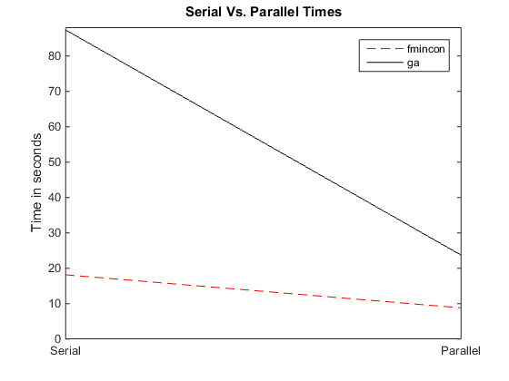
Utilizing parallel function evaluation via parfor improved the efficiency of both fmincon and ga. The improvement is typically better for expensive objective and constraint functions.
At last we delete the parallel pool.
if max(size(gcp)) > 0 % parallel pool exists
    delete(gcp) % delete the pool
end
Parallel pool using the 'local' profile is shutting down.