fmincon Interior-Point Algorithm with Analytic Hessian

The fmincon interior-point algorithm can accept a Hessian function as an input. When you supply a Hessian, you may obtain a faster, more accurate solution to a constrained minimization problem.

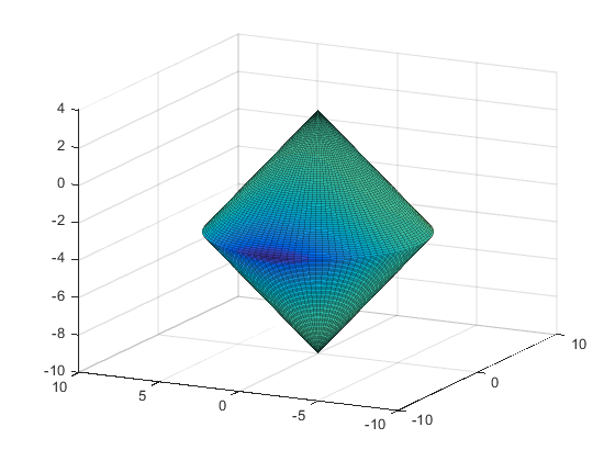
The constraint set for this example is the intersection of the interior of two cones—one pointing up, and one pointing down. The constraint function c is a two-component vector, one component for each cone. Since this is a three-dimensional example, the gradient of the constraint c is a 3-by-2 matrix.

function [c ceq gradc gradceq] = twocone(x)
% This constraint is two cones, z > -10 + r
% and z < 3 - r

ceq = [];
r = sqrt(x(1)^2 + x(2)^2);
c = [-10+r-x(3);
    x(3)-3+r];

if nargout > 2

    gradceq = [];
    gradc = [x(1)/r,x(1)/r;
       x(2)/r,x(2)/r;
       -1,1];

end

The objective function grows rapidly negative as the x(1) coordinate becomes negative. Its gradient is a three-element vector.

function [f gradf] = bigtoleft(x)
% This is a simple function that grows rapidly negative
% as x(1) gets negative
%
f=10*x(1)^3+x(1)*x(2)^2+x(3)*(x(1)^2+x(2)^2);

if nargout > 1

   gradf=[30*x(1)^2+x(2)^2+2*x(3)*x(1);
       2*x(1)*x(2)+2*x(3)*x(2);
       (x(1)^2+x(2)^2)];

end

Here is a plot of the problem. The shading represents the value of the objective function. You can see that the objective function is minimized near x = [-6.5,0,-3.5]:

Code for generating the figure

function createfigure2

% Create figure
figure1 = figure;

% Create axes
axes1 = axes('Parent',figure1);
view([-63.5 18]);
grid('on');
hold('all');

%Set up polar coordinates and two cones
r=0:.1:6.5;
th=2*pi*(0:.01:1);
x=r'*cos(th);
y=r'*sin(th);
z=-10+sqrt(x.^2+y.^2);
zz=3-sqrt(x.^2+y.^2);

%evaluate objective function on cone surfaces
newxf=reshape(bigtoleft2([reshape(x,6666,1),reshape(y,6666,1),reshape(z,6666,1)]),66,101)/3000;
newxg=reshape(bigtoleft2([reshape(x,6666,1),reshape(y,6666,1),reshape(zz,6666,1)]),66,101)/3000;

% Create lower surf with color set by objective
surf(x,y,z,newxf,'Parent',axes1,'EdgeAlpha',0.25);

% Create upper surf with color set by objective
surf(x,y,zz,newxg,'Parent',axes1,'EdgeAlpha',0.25);

The function bigtoleft2 is vectorized:

function f = bigtoleft2(x)
%
f=10*x(:,1).^3+x(:,1).*x(:,2).^2+x(:,3).*(x(:,1).^2+x(:,2).^2);

The Hessian of the Lagrangian is given by the equation:

$\nabla_{x x}^{2} L (x, λ) = \nabla^{2} f (x) + \sum λ_{i} \nabla^{2} c_{i} (x) + \sum λ_{i} \nabla^{2} c e q_{i} (x) .$

The following function computes the Hessian at a point x with Lagrange multiplier structure lambda:

function h = hessinterior(x,lambda)

h = [60*x(1)+2*x(3),2*x(2),2*x(1);
    2*x(2),2*(x(1)+x(3)),2*x(2);
    2*x(1),2*x(2),0];% Hessian of f
r = sqrt(x(1)^2+x(2)^2);% radius
rinv3 = 1/r^3;
hessc = [(x(2))^2*rinv3,-x(1)*x(2)*rinv3,0;
    -x(1)*x(2)*rinv3,x(1)^2*rinv3,0;
    0,0,0];% Hessian of both c(1) and c(2)
h = h + lambda.ineqnonlin(1)*hessc + lambda.ineqnonlin(2)*hessc;

Run this problem using the interior-point algorithm in fmincon. To do this using the Optimization app:

Set the problem as in the following figure.
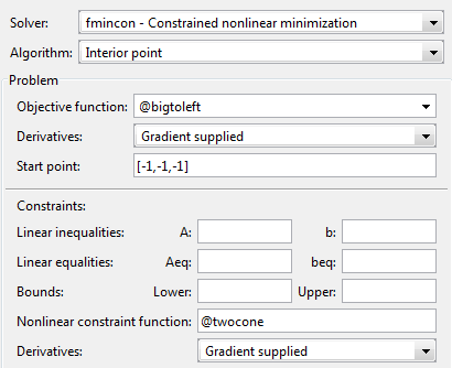
For iterative output, scroll to the bottom of the Options pane and select Level of display, iterative.
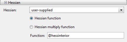
In the Options pane, give the analytic Hessian function handle.
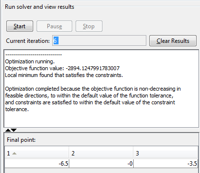
Under Run solver and view results, click Start.

To perform the minimization at the command line:

Set options as follows:

options = optimoptions(@fmincon,'Algorithm','interior-point',...
        'Display','off','GradObj','on','GradConstr','on',...
        'Hessian','user-supplied','HessFcn',@hessinterior);

Run fmincon with starting point [–1,–1,–1], using the options structure:

[x fval mflag output] = fmincon(@bigtoleft,[-1,-1,-1],...
           [],[],[],[],[],[],@twocone,options)

The output is:

x =
   -6.5000   -0.0000   -3.5000

fval =
  -2.8941e+03

mflag =
     1

output = 
         iterations: 6
          funcCount: 7
    constrviolation: 0
           stepsize: 3.0479e-05
          algorithm: 'interior-point'
      firstorderopt: 5.9812e-05
       cgiterations: 3
            message: 'Local minimum found that satisfies the constraints.…'

If you do not use a Hessian function, fmincon takes 9 iterations to converge, instead of 6:

options = optimoptions(@fmincon,'Algorithm','interior-point',...
        'Display','off','GradObj','on','GradConstr','on');

[x fval mflag output]=fmincon(@bigtoleft,[-1,-1,-1],...
           [],[],[],[],[],[],@twocone,options)

x =
   -6.5000   -0.0000   -3.5000

fval =
  -2.8941e+03

mflag =
     1

output = 
         iterations: 9
          funcCount: 13
    constrviolation: 2.9391e-08
           stepsize: 6.4842e-04
          algorithm: 'interior-point'
      firstorderopt: 1.4235e-04
       cgiterations: 0
            message: 'Local minimum found that satisfies the constraints.…'

Both runs lead to similar solutions, but the F-count and number of iterations are lower when using an analytic Hessian.

Related Examples

Was this topic helpful?

Documentation

fmincon Interior-Point Algorithm with Analytic Hessian

Related Examples

Optimization Toolbox Documentation

Other Documentation

Support