Documentation

This example shows how to generate and plot a Pareto front for a 2-D multiobjective function using fgoalattain.

The two objectives in this example are shifted and scaled versions of the convex function $$\sqrt{1+x^2}$$.

function f = simple_mult(x)

f(:,1) = sqrt(1+x.^2);
f(:,2) = 4 + 2*sqrt(1+(x-1).^2);

Both components are increasing as x decreases below 0 or increases above 1. In between 0 and 1, f₁(x) is increasing and f₂(x) is decreasing, so there is a tradeoff region.

t = linspace(-0.5,1.5);
F = simple_mult(t);
plot(t,F,'LineWidth',2)
hold on
plot([0,0],[0,8],'g--');
plot([1,1],[0,8],'g--');
plot([0,1],[1,6],'k.','MarkerSize',15);
text(-0.25,1.5,'Minimum(f_1(x))')
text(.75,5.5,'Minimum(f_2(x))')
hold off
legend('f_1(x)','f_2(x)')
xlabel({'x';'Tradeoff region between the green lines'})

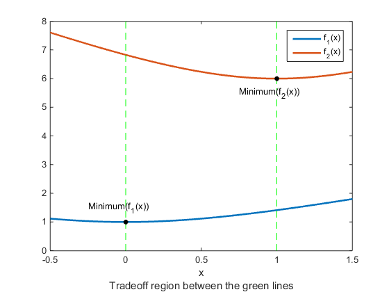
To find the Pareto front, first find the unconstrained minima of the two functions. In this case, you can see by inspection that the minimum of f₁(x) is 1, and the minimum of f₂(x) is 6, but in general you might need to use an optimization routine.

In general, write a function that returns a particular component of the multiobjective function.

function z = pickindex(x,k)
z = simple_mult(x); % evaluate both objectives
z = z(k); % return objective k

Then find the minimum of each component using an optimization solver. You can use fminbnd in this case, or fminunc for higher-dimensional problems.

k = 1;
[min1,minfn1] = fminbnd(@(x)pickindex(x,k),-1,2);
k = 2;
[min2,minfn2] = fminbnd(@(x)pickindex(x,k),-1,2);

Set goals that are the unconstrained optima for each component. You can simultaneously achieve these goals only if the multiobjective functions do not interfere with each other, meaning there is no tradeoff.

goal = [minfn1,minfn2];

To calculate the Pareto front, take weight vectors [a,1–a] for a from 0 through 1. Solve the goal attainment problem, setting the weights to the various values.

nf = 2; % number of objective functions
N = 50; % number of points for plotting
onen = 1/N;
x = zeros(N+1,1);
f = zeros(N+1,nf);
fun = @simple_mult;
x0 = 0.5;
options = optimoptions('fgoalattain','Display','off');
for r = 0:N
    t = onen*r; % 0 through 1
    weight = [t,1-t];
    [x(r+1,:),f(r+1,:)] = fgoalattain(fun,x0,goal,weight,...
        [],[],[],[],[],[],[],options);
end

figure
plot(f(:,1),f(:,2),'k.');
xlabel('f_1')
ylabel('f_2')

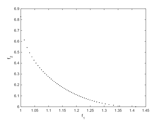
You can see the tradeoff between the two objectives.