Mixed-Integer Quadratic Programming Portfolio Optimization
This example shows how to solve a Mixed-Integer Quadratic Programming (MIQP) portfolio optimization problem using the intlinprog Mixed-Integer Linear Programming (MILP) solver. The idea is to iteratively solve a sequence of MILP problems that locally approximate the MIQP problem.
Problem Outline
As Markowitz showed ("Portfolio Selection," J. Finance Volume 7, Issue 1, pp. 77-91, March 1952), you can express many portfolio optimization problems as quadratic programming problems. Suppose that you have a set of N assets and want to choose a portfolio, with
 being the fraction of your investment that is in asset
 . If you know the vector
 of mean returns of each asset, and the covariance matrix
 of the returns, then for a given level of risk-aversion
 you maximize the risk-adjusted expected return:
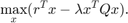
The quadprog solver addresses this quadratic programming problem. However, in addition to the plain quadratic programming problem, you might want to restrict a portfolio in a variety of ways, such as:
Having no more than
Massets in the portfolio, whereM <= N.Having at least
massets in the portfolio, where0 < m <= M.Having semicontinuous constraints, meaning either
 , or
, or
 for some fixed fractions
 and
and
 .
.
You cannot include these constraints in quadprog. The difficulty is the discrete nature of the constraints. Furthermore, while the mixed-integer linear programming solver intlinprog does handle discrete constraints, it does not address quadratic objective functions.
This example constructs a sequence of MILP problems that satisfy the constraints, and that increasingly approximate the quadratic objective function. While this technique works for this example, it might not apply to different problem or constraint types.
Begin by modeling the constraints.
Modeling Discrete Constraints
 is the vector of asset allocation fractions, with
 for each
. To model the number of assets in the portfolio, you need indicator variables
for each
. To model the number of assets in the portfolio, you need indicator variables
 such that
 when
, and
when
, and
 when
when
 . To get variables that satisfy this restriction, set the
vector to be a binary variable, and impose the linear constraints
. To get variables that satisfy this restriction, set the
vector to be a binary variable, and impose the linear constraints

These inequalities both enforce that
and
 are zero at exactly the same time, and they also enforce that
 whenever
.
whenever
.
Also, to enforce the constraints on the number of assets in the portfolio, impose the linear constraints
Objective and Successive Linear Approximations
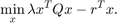
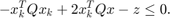
As first formulated, you try to maximize the objective function. However, all Optimization Toolbox™ solvers minimize. So formulate the problem as minimizing the negative of the objective:
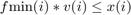
This objective function is nonlinear. The intlinprog MILP solver requires a linear objective function. There is a standard technique to reformulate this problem into one with linear objective and nonlinear constraints. Introduce a slack variable
 to represent the quadratic term.

As you iteratively solve MILP approximations, you include new linear constraints, each of which approximates the nonlinear constraint locally near the current point. In particular, for
 where
where
 is a constant vector and
 is a variable vector, the first-order Taylor approximation to the constraint is

Replacing
by
 gives
gives

For each intermediate solution
 you introduce a new linear constraint in
and
as the linear part of the expression above:
you introduce a new linear constraint in
and
as the linear part of the expression above:
This has the form
 , where
 , there is a
 multiplier for the
term, and
multiplier for the
term, and
 .
.
This method of adding new linear constraints to the problem is called a cutting plane method. For details, see J. E. Kelley, Jr. "The Cutting-Plane Method for Solving Convex Programs." J. Soc. Indust. Appl. Math. Vol. 8, No. 4, pp. 703-712, December, 1960.
MATLAB® Problem Formulation
To express problems for the intlinprog solver, you need to do the following:
Decide what your variables represent
Express lower and upper bounds in terms of these variables
Give linear equality and inequality matrices
Have the first
 variables represent the
vector, the next
variables represent the binary
vector, and the final variable represent the
slack variable. There are
variables represent the
vector, the next
variables represent the binary
vector, and the final variable represent the
slack variable. There are
 variables in the problem.
Load the data for the problem. This data has 225 expected returns in the vector r and the covariance of the returns in the 225-by-225 matrix Q. The data is the same as in the Using Quadratic Programming on Portfolio Optimization Problems example.
load port5
r = mean_return;
Q = Correlation .* (stdDev_return * stdDev_return');
Set the number of assets as N.
N = length(r);
Set indexes for the variables
xvars = 1:N;
vvars = N+1:2*N;
zvar = 2*N+1;
The lower bounds of all the 2N+1 variables in the problem are zero. The upper bounds of the first 2N variables are one, and the last variable has no upper bound.
lb = zeros(2*N+1,1);
ub = ones(2*N+1,1);
ub(zvar) = Inf;
Set the number of assets in the solution to be between 100 and 150. Incorporate this constraint into the problem in the form, namely
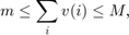
by writing two linear constraints of the form
 :
:

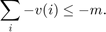
M = 150;
m = 100;
A = zeros(1,2*N+1); % Allocate A matrix
A(vvars) = 1; % A*x represents the sum of the v(i)
A = [A;-A];
b = zeros(2,1); % Allocate b vector
b(1) = M;
b(2) = -m;
Include semicontinuous constraints. Take the minimal nonzero fraction of assets to be 0.001 for each asset type, and the maximal fraction to be 0.05.
fmin = 0.001;
fmax = 0.05;
Include the inequalities
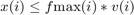 and
and
 as linear inequalities.
Atemp = eye(N);
Amax = horzcat(Atemp,-Atemp*fmax,zeros(N,1));
A = [A;Amax];
b = [b;zeros(N,1)];
Amin = horzcat(-Atemp,Atemp*fmin,zeros(N,1));
A = [A;Amin];
b = [b;zeros(N,1)];
Include the constraint that the portfolio is 100% invested, meaning
 .
.
Aeq = zeros(1,2*N+1); % Allocate Aeq matrix
Aeq(xvars) = 1;
beq = 1;
Set the risk-aversion coefficient
to 100.
lambda = 100;
Define the objective function
 as a vector. Include zeros for the multipliers of the
variables.
as a vector. Include zeros for the multipliers of the
variables.
f = [-r;zeros(N,1);lambda];
Solve the Problem
To solve the problem iteratively, begin by solving the problem with the current constraints, which do not yet reflect any linearization. The integer constraints are in the vvars vector.
options = optimoptions(@intlinprog,'Display','off'); % Suppress iterative display
[xLinInt,fval,exitFlagInt,output] = intlinprog(f,vvars,A,b,Aeq,beq,lb,ub,options);
Prepare a stopping condition for the iterations: stop when the slack variable
is within 0.01% of the true quadratic value.
thediff = 1e-4;
iter = 1; % iteration counter
assets = xLinInt(xvars); % the x variables
truequadratic = assets'*Q*assets;
zslack = xLinInt(zvar); % slack variable value
Keep a history of the computed true quadratic and slack variables for plotting.
history = [truequadratic,zslack];
Compute the quadratic and slack values. If they differ, then add another linear constraint and solve again.
In toolbox syntax, each new linear constraint
comes from the linear approximation
You see that the new row of
and the new element in
, with the
term represented by a -1 coefficient in
 .
.
After you find a new solution, use a linear constraint halfway between the old and new solutions. This heuristic way of including linear constraints can be faster than simply taking the new solution. To use the solution instead of the halfway heuristic, comment the "Midway" line below, and uncomment the following one.
while abs((zslack - truequadratic)/truequadratic) > thediff % relative error
    newArow = horzcat(2*assets'*Q,zeros(1,N),-1); % Linearized constraint
    A = [A;newArow];
    b = [b;truequadratic];
    % Solve the problem with the new constraints
    [xLinInt,fval,exitFlagInt,output] = intlinprog(f,vvars,A,b,Aeq,beq,lb,ub,options);
    assets = (assets+xLinInt(xvars))/2; % Midway from the previous to the current
%     assets = xLinInt(xvars); % Use the previous line or this one
    truequadratic = assets'*Q*assets;
    zslack = xLinInt(zvar);
    history = [history;truequadratic,zslack];
    iter = iter + 1;
end
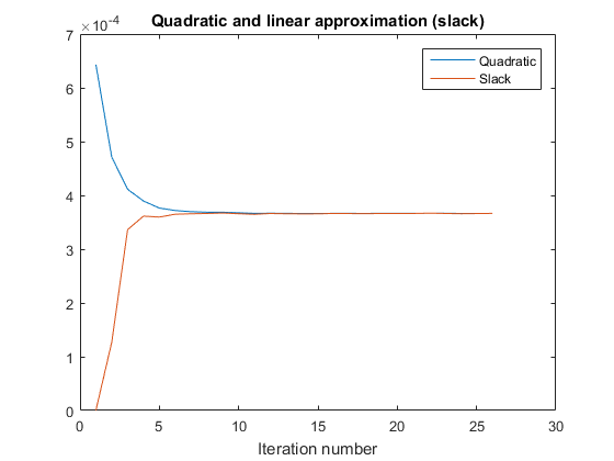
Examine the Solution and Convergence Rate
Plot the history of the slack variable and the quadratic part of the objective function to see how they converged.
plot(history)
legend('Quadratic','Slack')
xlabel('Iteration number')
title('Quadratic and linear approximation (slack)')
What is the quality of the MILP solution? The output structure contains that information. Examine the absolute gap between the internally-calculated bounds on the objective at the solution.
disp(output.absolutegap)
0
The absolute gap is zero, indicating that the MILP solution is accurate.
Plot the optimal allocation. Use xLinInt(xvars), not assets, because assets might not satisfy the constraints when using the midway update.
bar(xLinInt(xvars))
grid on
xlabel('Asset index')
ylabel('Proportion of investment')
title('Optimal asset allocation')
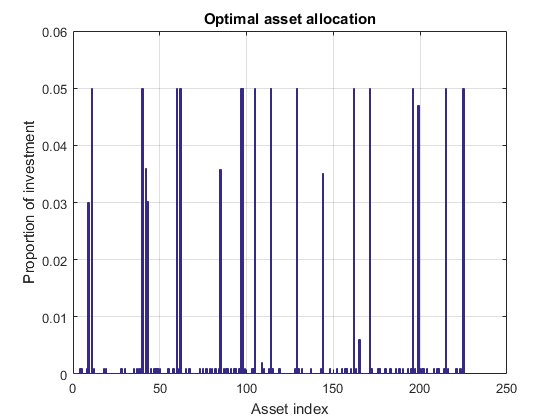
You can easily see that all nonzero asset allocations are between the semicontinuous bounds
 and
and
 .
.
How many nonzero assets are there? The constraint is that there are between 100 and 150 nonzero assets.
sum(xLinInt(vvars))
ans =

   100
What is the expected return for this allocation, and the value of the risk-adjusted return?
fprintf('The expected return is %g, and the risk-adjusted return is %g.\n',...
    r'*xLinInt(xvars),-fval)
The expected return is 0.000616464, and the risk-adjusted return is -0.0360334.
More elaborate analyses are possible by using features specifically designed for portfolio optimization in Financial Toolbox™.