Documentation

This example shows how to use the Optimization app with the fmincon solver to minimize a quadratic subject to linear and nonlinear constraints and bounds.

Note:   The Optimization app warns that it will be removed in a future release.

Consider the problem of finding [x₁, x₂] that solves

$$\underset{x}{\min }f(x)=x_1^2+x_2^2$$

subject to the constraints

$$\begin{array}{rr}\hfill 0.5\le x_1& \hfill \text{(bound)}\\ \hfill -x_1-x_2+1\le 0& \hfill \text{(linear inequality)}\\ \hfill \begin{array}{r}\hfill -x_1^2-x_2^2+1\le 0\\ \hfill -9x_1^2-x_2^2+9\le 0\\ \hfill -x_1^2+x_2\le 0\\ \hfill -x_2^2+x_1\le 0\end{array}\}& \hfill \text{(nonlinear inequality)}\end{array}$$

The starting guess for this problem is x₁ = 3 and x₂ = 1.

Step 1: Write a file objecfun.m for the objective function.

function f = objecfun(x)
f = x(1)^2 + x(2)^2;

Step 2: Write a file nonlconstr.m for the nonlinear constraints.

function [c,ceq] = nonlconstr(x)
c = [-x(1)^2 - x(2)^2 + 1;
     -9*x(1)^2 - x(2)^2 + 9;
     -x(1)^2 + x(2);
     -x(2)^2 + x(1)];
ceq = [];

Step 3: Set up and run the problem with the Optimization app.

1. Enter optimtool in the Command Window to open the Optimization app.

2. Select fmincon from the selection of solvers and change the Algorithm field to Active set.

   

3. Enter @objecfun in the Objective function field to call the objecfun.m file.

4. Enter [3;1] in the Start point field.

   

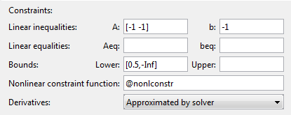
5. Define the constraints.

   • Set the bound 0.5 ≤ x₁ by entering [0.5,-Inf] in the Lower field. The -Inf entry means there is no lower bound on x₂.

   • Set the linear inequality constraint by entering [-1 -1] in the A field and enter -1 in the b field.

   • Set the nonlinear constraints by entering @nonlconstr in the Nonlinear constraint function field.

   

6. In the Options pane, expand the Display to command window option if necessary, and select Iterative to show algorithm information at the Command Window for each iteration.

   

7. Click the Start button as shown in the following figure.

   

8. When the algorithm terminates, under Run solver and view results the following information is displayed:

   

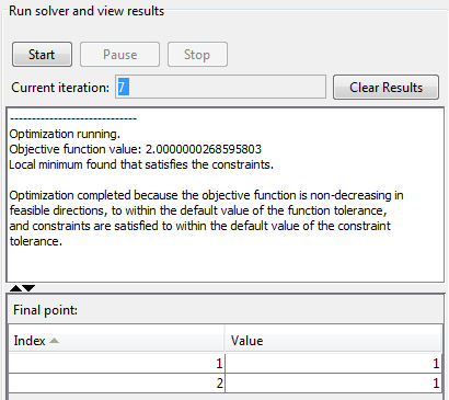
   • The Current iteration value when the algorithm terminated, which for this example is 7.

   • The final value of the objective function when the algorithm terminated:

     Objective function value: 2.0000000268595803

   • The algorithm termination message:

     Local minimum found that satisfies the constraints.
     
     Optimization completed because the objective function is non-decreasing in 
     feasible directions, to within the default value of the function tolerance,
     and constraints are satisfied to within the default value of the constraint tolerance.

   • The final point, which for this example is

         1
         1	

9. In the Command Window, the algorithm information is displayed for each iteration:

                                Max   Line search  Directional  First-order 
   Iter F-count     f(x)  constraint steplength   derivative   optimality Procedure 
      0     3        10            2                            Infeasible start point
      1     6   4.84298      -0.1322       1      -5.22       1.74   
      2     9    4.0251     -0.01168       1      -4.39       4.08  Hessian modified twice  
      3    12   2.42704     -0.03214       1      -3.85       1.09   
      4    15   2.03615    -0.004728       1      -3.04      0.995  Hessian modified twice  
      5    18   2.00033  -5.596e-005       1      -2.82     0.0664  Hessian modified twice  
      6    21         2  -5.327e-009       1      -2.81   0.000522  Hessian modified twice  
   
   Local minimum found that satisfies the constraints.
   
   Optimization completed because the objective function is non-decreasing in 
   feasible directions, to within the default value of the function tolerance,
   and constraints are satisfied to within the default value of the constraint tolerance.
   
   Active inequalities (to within options.TolCon = 1e-006):
     lower      upper     ineqlin   ineqnonlin
                                        3
                                        4