# Graphs #
In this Chapter we will learn how to exploit some of the functionalities
that ROOT provides to display data exploiting the class `TGraphErrors`,
which you already got to know previously.
## Read Graph Points from File ##
The fastest way in which you can fill a graph with experimental data is
to use the constructor which reads data points and their errors from a
file in ASCII (i.e. standard text) format:
``` {.cpp}
TGraphErrors(const char *filename,
const char *format="%lg %lg %lg %lg", Option_t *option="");
```
The format string can be:
- `"\%lg \%lg"` read only 2 first columns into X,Y
- `"\%lg \%lg \%lg"` read only 3 first columns into X,Y and EY
- `"\%lg \%lg \%lg \%lg"` read only 4 first columns into X,Y,EX,EY
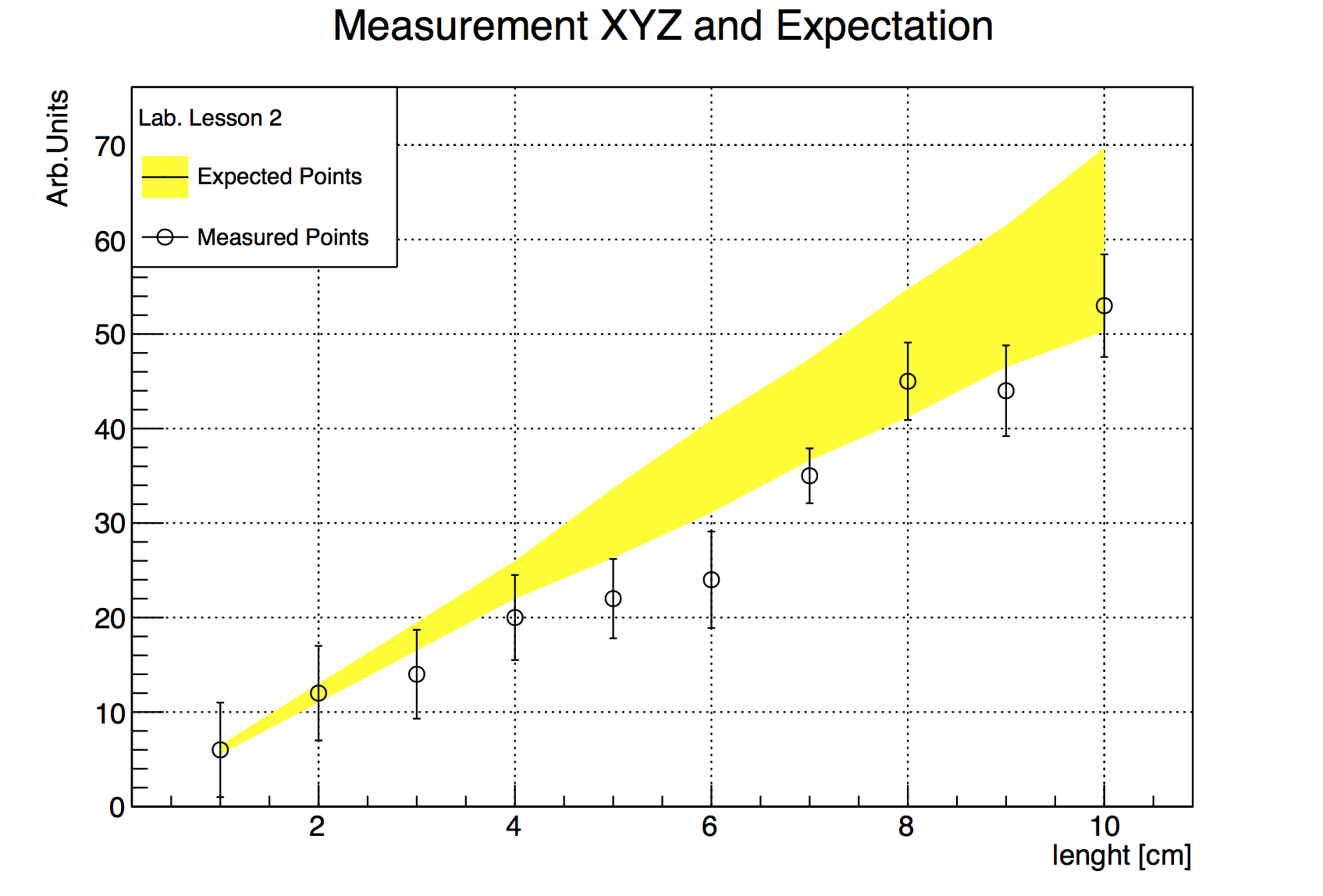
This approach has the nice feature of allowing the user to reuse the
macro for many different data sets. Here is an example of an input file.
The nice graphic result shown is produced by the macro below, which
reads two such input files and uses different options to display the
data points.
```
# Measurement of Friday 26 March
# Experiment 2 Physics Lab
1 6 5
2 12 5
3 14 4.7
4 20 4.5
5 22 4.2
6 24 5.1
7 35 2.9
8 45 4.1
9 44 4.8
10 53 5.43
```
``` {.cpp}
// Reads the points from a file and produces a simple graph.
int macro2(){
TCanvas* c=new TCanvas();
c->SetGrid();
TGraphErrors graph_expected("./macro2_input_expected.txt",
"%lg %lg %lg");
graph_expected.SetTitle(
"Measurement XYZ and Expectation;
lenght [cm];
Arb.Units");
graph_expected.SetFillColor(kYellow);
graph_expected.DrawClone("E3AL"); // E3 draws the band
TGraphErrors graph("./macro2_input.txt","%lg %lg %lg");
graph.SetMarkerStyle(kCircle);
graph.SetFillColor(0);
graph.DrawClone("PESame");
// Draw the Legend
TLegend leg(.1,.7,.3,.9,"Lab. Lesson 2");
leg.SetFillColor(0);
leg.AddEntry(&graph_expected,"Expected Points");
leg.AddEntry(&graph,"Measured Points");
leg.DrawClone("Same");
graph.Print();
}
```
In addition to the inspection of the plot, you can check the actual
contents of the graph with the `TGraph::Print()` method at any time,
obtaining a printout of the coordinates of data points on screen. The
macro also shows us how to print a coloured band around a graph instead
of error bars, quite useful for example to represent the errors of a
theoretical prediction.
## Polar Graphs ##
With ROOT you can profit from rather advanced plotting routines, like
the ones implemented in the `TPolarGraph`, a class to draw graphs in
polar coordinates. It is very easy to use, as you see in the example
macro and the resulting Figure [4.1](#f41):
``` {.cpp .numberLines}
// Builds a polar graph in a square Canvas.
void macro3(){
TCanvas* c = new TCanvas("myCanvas","myCanvas",600,600);
double rmin=0;
double rmax=TMath::Pi()*6;
const int npoints=1000;
Double_t r[npoints];
Double_t theta[npoints];
for (Int_t ipt = 0; ipt < npoints; ipt++) {
r[ipt] = ipt*(rmax-rmin)/npoints+rmin;
theta[ipt] = TMath::Sin(r[ipt]);
}
TGraphPolar grP1 (npoints,r,theta);
grP1.SetTitle("A Fan");
grP1.SetLineWidth(3);
grP1.SetLineColor(2);
grP1.DrawClone("AOL");
}
```
A new element was added on line 4, the size of the canvas: it is
sometimes optically better to show plots in specific canvas sizes.
[f41]: figures/polar_graph.png "f41"
![The graph of a fan obtained with ROOT.\label{f41}][f41]
## 2D Graphs ##
Under specific circumstances, it might be useful to plot some quantities
versus two variables, therefore creating a bi-dimensional graph. Of
course ROOT can help you in this task, with the `TGraph2DErrors` class.
The following macro produces a bi-dimensional graph representing a
hypothetical measurement, fits a bi-dimensional function to it and draws
it together with its x and y projections. Some points of the code will
be explained in detail. This time, the graph is populated with data
points using random numbers, introducing a new and very important
ingredient, the ROOT `TRandom3` random number generator using the
Mersenne Twister algorithm [@MersenneTwister].
``` {.cpp .numberLines}
// Create, Draw and fit a TGraph2DErrors
void macro4(){
gStyle->SetPalette(1);
const double e = 0.3;
const int nd = 500;
TRandom3 my_random_generator;
TF2 *f2 = new TF2("f2",
"1000*(([0]*sin(x)/x)*([1]*sin(y)/y))+200",
-6,6,-6,6);
f2->SetParameters(1,1);
TGraph2DErrors *dte = new TGraph2DErrors(nd);
// Fill the 2D graph
double rnd, x, y, z, ex, ey, ez;
for (Int_t i=0; iGetRandom2(x,y);
// A random number in [-e,e]
rnd = my_random_generator.Uniform(-e,e);
z = f2->Eval(x,y)*(1+rnd);
dte->SetPoint(i,x,y,z);
ex = 0.05*my_random_generator.Uniform();
ey = 0.05*my_random_generator.Uniform();
ez = TMath::Abs(z*rnd);
dte->SetPointError(i,ex,ey,ez);
}
// Fit function to generated data
f2->SetParameters(0.7,1.5); // set initial values for fit
f2->SetTitle("Fitted 2D function");
dte->Fit(f2);
// Plot the result
TCanvas *c1 = new TCanvas();
f2->Draw("Surf1");
dte->Draw("P0 Same");
// Make the x and y projections
TCanvas* c_p= new TCanvas("ProjCan",
"The Projections",1000,400);
c_p->Divide(2,1);
c_p->cd(1);
dte->Project("x")->Draw();
c_p->cd(2);
dte->Project("y")->Draw();
}
```
Let's go through the code, step by step to understand what is going on:
- Line *3*: This sets the palette colour code to a much nicer one than
the default. Comment this line to give it a try.
- Line *7*: The instance of the random generator. You can then draw
out of this instance random numbers distributed according to
different probability density functions, like the Uniform one at
lines *27-29*. See the on-line documentation to appreciate the full
power of this ROOT feature.
- Line *12*: You are already familiar with the `TF1` class. This is
its two-dimensional correspondent. At line *24* two random numbers
distributed according to the `TF2` formula are drawn with the method
`TF2::GetRandom2(double& a, double&b)`.
- Line *27-29*: Fitting a 2-dimensional function just works like in
the one-dimensional case, i.e. initialisation of parameters and
calling of the `Fit()` method.
- Line *32*: The *Surf1* option draws the `TF2` objects (but also
bi-dimensional histograms) as coloured surfaces with a wire-frame on
three-dimensional canvases. See Figure [4.2](#f42).
- Line *37-41*: Here you learn how to create a canvas, partition it in
two sub-pads and access them. It is very handy to show multiple
plots in the same window or image.
[f42]: figures/fitted2dFunction.png "f42"
![A dataset fitted with a bidimensional function visualised as a colored
surface.\label{f42}][f42]