Module: Absolute Permeability Experiment Simulation ()

Description:

The Absolute Permeability Experiment Simulation module simulates an experiment leading to the computation of absolute permeability.

Note: see about system requirements and hardware platform availability.

Aknowledgments

This module was developed in collaboration with Dominique Bernard, Research Director at ICMCB-CNRS (Pessac, France).

Theoritical details

Some general elements about absolute permeability are exposed in . More precisely, the Stokes problem is solved by imposing boundary conditions:

• one voxel wide plane of solid phase is added on the faces of the image that are not perpendicular to the main flow direction. This allows isolating the sample from the outside, letting no flow to go out of the system;
• experimental setups are added on the faces of the image that are perpendicular to the main flow direction. They are designed in a manner that creates a stabilization zone where pressure is quasi static, and the fluid can freely spread on the input face of the sample.
• two among the following three conditions can be chosen by the user, the third being estimated from the chosen two: input pressure, output pressure, flow rate.

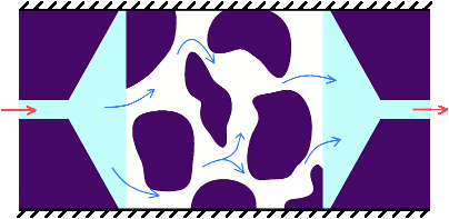
Input pressure is imposed at the entrance of the experimental setup, as long as output pressure is imposed at the exit of the experimental setup. Flow rate is guaranteed to remain the same at entrance and exit as the sample is hermetically enclosed by solid. Absolute permeability is obtained by a simple application of Darcy's law.

Physical constraints

The absolute permeability is computed with a single-phase flow. The module takes a labeled image as input, but each label of the image has to be part either of the solid or of the fluid phase: only one solid and one fluid phase are considered for this calculation. The solid phase is impermeable: there is no flow in it.

Computational aspects and results

As the computation can be rather long, it is left to the user to select whether one or several experiments must be computed. The results are presented in a spreadsheet with suffix .KExp.Spreadsheet. There is one table for each direction (X, Y and Z).

Each line of the spreadsheet represents a single computation of the property. The columns contain:

• Geometry file: name of the file on which the computation was done;
• Region of interest: bounding box of the ROI on which the computation was performed;
• k: value of the absolute permeability of the sample in square micrometer;
• k: value of the absolute permeability of the sample in darcy.

Units and dimensions

The boundary conditions (input pressure, output pressure, flow rate) are supposed to be in [] for the pressures and in [] for the flow rates. The viscosity is in [].

The permeability results are presented on two columns: the first is in , the second in . The values are very close since 1 darcy, a common unit for permeability, almost equals 1 (1 = 0,9869233 ).

Problems and solutions

What does this error dialog mean?

Figure 1: Example of error dialog at the end of a computation.

This dialog usually appears at the end of a computation and means that something went wrong during the computation. The solver did not reach the convergence target in the indicated number of iterations. There can be mainly two reasons to explain that problem.

First, the number of iterations is not large enough. It can be detected when the performed number of iterations equals the maximal number set as parameter. The maximal limit should be increased in the parameters of the modules. For large data volumes, the default value might be too small.

The other reason is more difficult to identify. When the discretization of the volume is too rough, the solver can start oscillating locally. One value is locally perturbed and each iteration modifies it consequently with respect to its absolute value. This value can be very small but the error is computed on relative variation between two time steps. For example, a value of at iteration number 1 and at iteration 2 varied by between these two iterations. The value is very small, probably negligible for the final result, but the error remains large.

Several solutions can be tested to address these issues:

• Try to remove the non-percolating porosity from the input image. Non-percolating porosity is not involved in the physical property, but computation in it can be rather long to finally end to 0. To remove this porosity, the Axis Connectivity module can be used. The can help to apply this processing.
• Reduce the convergence criterion value, so that the solver iterates longer and reaches a lower error value. Also increase the maximum number of iteration, so that the solver is not bound by that number.
• Try to increase the refining coefficient. This parameter is hidden by default in the XLab modules parameters. To modify it, the Advanced Settings checkbox must be selected, then a slider appears below the list of materials. Setting refining coefficient to 2 means that all voxels is divided by 2 in the three directions of space. On one hand, it multiplies the number of unknowns to compute (probably memory consumption and computation time also) by a factor of 8. On the other hand, it increases the numeric precision and often helps the solver to converge when it could not with a refining coefficient of 1.

Note: The GPU-accelerated version of this module requires a CUDA-enabled GPU. All compatible GPUs are listed here. The current implementation of this module uses only one GPU.

Connections:

Data [required]
The input must be a Label Field.

ROI [optional]
This is a Region Of Interest, meaning that the computation will only take into account the volume contained in the ROI.

Initial Velocity Field [optional]

Initial Pressure Field [optional]
The connected fields are used as initial solution of the problem. It means that the result of a previous computation can be reused to restart this computation from where it ended. It can be useful if the computation was interrupted before the targeted error value was reached. Both fields must be connected, otherwise no initialization will be used. Initializing only velocities or pressures does not allow restarting the computation in an efficient way. The connected fields must have the same dimensions and voxel size as the data set. Otherwise, they will not be used for initializing the solution.

Ports:

Options

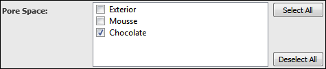
This checkbox allows overwriting (checked) / creating new outputs (unchecked) when a computation ends.

Pore Space

This port lists all the materials or labels contained in the connected Label Field. It allows selecting which labels or values must be considered as fluid for the computation. By default, the material named Exterior or the value 0 is selected.

Direction

This option allows the user to define the direction of main flow. Separate computations will be performed for each direction specified.

Spreadsheet

This port selects where the next result must appear. If "append result" is selected, the next result is appended in the connected spreadsheet to the last created table corresponding to the species transport direction of this computation. If "new spreadsheet" is selected, the result is stored in a new spreadsheet. If no spreadsheet is connected, a new one is created.

Outputs

If one of the check boxes is selected, the corresponding output will appear in the Project View at the end of the computation. The two first check boxes stand for the resulting velocity and pressure fields. They are selected by default.

The third check box is checked by default. If the box is checked, a spreadsheet with suffix .KExp.Error.Spreadsheet is added to the Project View. It contains the estimation of the error (or convergence criterion) at each iteration, for each computation (depending on how many directions are selected).

Note: the velocity and pressure fields are automatically created as output of the module if the computation was aborted or did not converge. The created fields can be connected as inputs of the module, so that the computed values can be used as initial solution of the problem (see above for more details).

Boundary Conditions

This port allows choosing the two boundary conditions to be imposed to the experimental system. The choices are "input pressure + output pressure", "input pressure + flow rate" and "output pressure + flow rate". A change on this port is detected for the port "Boundary values" and for the calculation of the final result.

Note: absolute permeability is independent from boundary conditions. Only velocity and pressure fields are rescaled according to boundary conditions.

Boundary Values

These are the values corresponding to the selected conditions "Boundary conditions". The labels of the text fields are modified depending on the boundary conditions. The units to use for pressure are Pa and for flow rate. These values are used for scaling the velocity and pressure fields.

Note: absolute permeability is independent from boundary conditions. Only velocity and pressure fields are rescaled according to the indicated values.

Fluid Viscosity

Value of the viscosity of the fluid used for experiment simulation (in ) The viscosity must be positive in the computation, since the considered fluids are Newtonian.

Note: absolute permeability is independent from boundary conditions. Only velocity and pressure fields are rescaled according to fluid viscosity.

hxportgroup Compute Device

Compute Device

This port allows choosing the device for the next computation.

If CPU is selected, the computation will use the number of threads defined in the Preferences Performance. CPU is always available.

If GPU is selected, the port CUDA Device appears. GPU could not be selected for some hardware configuration (see below) and is then insensitive.

Note: The GPU-accelerated version of this module requires a CUDA-enabled GPU. All compatible GPUs are listed here. The current implementation of this module uses only one GPU.

CUDA Device

This port shows a list of all the CUDA devices that can be used for the computation. It is visible only if:

• the graphics driver is recent enough to support CUDA computing;
• the license was found ();
• at least one of the existing device has a compute capability greater than or equal to 2.0.

Each line of this port shows the name of the device, an identifier and the total amount of memory available. These information could help choosing the best device for computation.

Warning

This port is shown only when a message needs to be displayed:

• if an insufficient driver, which is not supporting CUDA, is detected;
• if no CUDA device is detected on the hardware;
• if the necessary license is incorrectly detected;
• if none of the existing devices has a compute capability greater than or equal to 2.0.

Otherwise, this port is not visible.

hxportgroup Advanced Settings

Advanced Settings

This port sets whether the additional options for fine tuning the module are visible (ON) or hidden (OFF). The options that appear when switching ON are considered to be expert options, which should not require modification in most cases.

Refining Coefficient

Only appears when "show advanced settings" from port Options is checked. The refining coefficient can be used to artificially oversample an image, by simply dividing all the voxels by an integer value. This method gives better precision concerning the evaluation of the unknowns. It can be useful to increase it when the throats in the porous materials are very small (few voxels wide). It is an integer value, which must be strictly greater than 0. The slider is limited to 2 to avoid an accidental increase of this value, which would imply a heavy increase of unknown numbers, though a dramatic drop in computation time.

Convergence Criterion

Only appears when "show advanced settings" from port Options is checked. It is assumed that convergence is attained when the time derivatives of the unknowns tend to 0. To evaluate this behavior, the convergence criterion is computed as:

where is the current iteration, is the velocity vector, is the pressure field, is the time step and is the artificial compressibility coefficient (please refer to for more details). Numerically, 0 can never be reached; that is why a precision value must be set to indicate that the convergence is sufficient. This is a floating point value which must be greater than 0 and for which a default value of 10 is suggested.

Warning: the default value is not appropriate for any computation. Depending on the geometry of the sample, it might be mandatory to decrease the precision value drastically.

For convenience, the convergence criterion will often be simply called "error" in the GUI, spreadsheets and Console messages.

Iterations

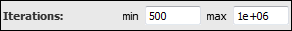
Only appears when "show advanced settings" from port Options is checked. It is important to know that an explicit resolution is used to solve the Stokes equation system for the permeability computation. There are two numbers to set in this port. The first is the minimum number of iterations to compute. It is used to avoid ending the computation loop too early. It could happen in very specific cases, due to numerical oscillation in the first iterations. These oscillations can sometimes make the time derivative falsely lower than the convergence criterion. The second number refers to the maximum number of iterations to compute. It is used to be sure that the computation loop will end even if the convergence criterion cannot be attained because of numerical approximation problems. Each number can be set to a default value that should be enough for most cases. A computation should not need more than 100 000 iterations, which already is a huge value. The oscillations should not remain beyond 500 iterations.

Expose

This port stands for the refined image. The output that is shown in the Project View is the refined subvolume used for the computation. It means that the output field fits in the ROI if it is defined or has the same dimensions as the input data. It also means that the output field is oversampled by the factor indicated in the refining coefficient option.