Module: Thermal Conductivity Experiment Simulation ()

Description:

The Thermal Conductivity Experiment Simulation module simulates an experiment leading to the computation of the thermal conductivity of a material.

Note: see about system requirements and hardware platform availability.

Aknowledgments

This module was developed in collaboration with Dominique Bernard, Research Director at ICMCB-CNRS (Pessac, France).

Theoritical details

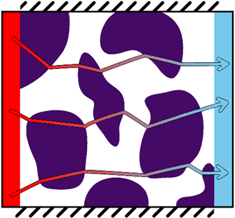
Some general elements about thermal conductivity are exposed in . More precisely, the transport equation is solved by imposing boundary conditions:

• one voxel wide plane of thermal insulator is added on the faces of the image that are not perpendicular to the heat flux main direction. This allows isolating the sample from the outside.
• the input and output (the faces that are perpendicular to the flux main direction) are designed as one voxel wide planes where the temperature is imposed.
• two among the following three conditions can be imposed by the user, the third being estimated from the chosen two: input temperature, output temperature, heat flux.
• the temperature and the normal component of the heat flux are continuous at the interface between two conducting phases.

Physical constraints

The sample considered might be composed of several phases. The module takes a label image as input and the user has to provide the thermal conductivity for each label corresponding to a phase that is conducting heat. The other phases (labels) are considered as thermal insulators: there is no heat flux in them and their thermal conductivity is null.

Computational aspects and results

As the computation can be rather long, it is left to the user to select whether one or several experiments must be computed. The results are presented in a spreadsheet with suffix .TCExp.Spreadsheet.

There is one table for each direction (X, Y and Z). Each line of the spreadsheet represents a single computation of the properties. The columns contain:

• Geometry file: name of the file on which the computation was performed,
• Region of interest: bounding box of the ROI on which the computation was performed,
• Apparent thermal conductivity: value of the thermal conductivity of the sample in [],
• Material thermal conductivity: thermal conductivity for each heat conducting phase of the sample in [].

Units and dimensions

The input and output temperature boundary conditions are supposed to be in []. The thermal conductivities are expressed in []. The heat flux is expressed in [].

Problems and solutions

What does this error dialog mean?

Figure 1: Example of error dialog at the end of a computation.

This dialog usually appears at the end of a computation and means that something went wrong during the computation. The solver did not reach the convergence target in the indicated number of iterations. There can be mainly two reasons to explain that problem.

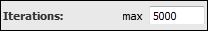
First, the number of iterations is not large enough. It can be detected when the performed number of iterations equals the maximal number set as parameter. The maximal limit should be increased in the parameters of the modules. For large data volumes, the default value might be too small.

The other reason is more difficult to identify. When the discretization of the volume is too rough, the solver can start oscillating locally. One value is locally perturbed and each iteration modifies it consequently with respect to its absolute value. This value can be very small but the error is computed on relative variation between two time steps. For example, a value of at iteration number 1 and at iteration 2 varied by between these two iterations. The value is very small, probably negligible for the final result, but the error remains large.

Several solutions can be tested to address these issues:

• Try to remove the non-percolating porosity from the input image. Non-percolating porosity is not involved in the physical property, but computation in it can be rather long to finally end to 0. To remove this porosity, the Axis Connectivity module can be used. The can help to apply this processing.
• Reduce the convergence criterion value, so that the solver iterates longer and reaches a lower error value. Also increase the maximum number of iteration, so that the solver is not bound by that number.
• Try to increase the refining coefficient. This parameter is hidden by default in the XLab modules parameters. To modify it, the Advanced Settings checkbox must be selected, then a slider appears below the list of materials. Setting refining coefficient to 2 means that all voxels is divided by 2 in the three directions of space. On one hand, it multiplies the number of unknowns to compute (probably memory consumption and computation time also) by a factor of 8. On the other hand, it increases the numeric precision and often helps the solver to converge when it could not with a refining coefficient of 1.

Connections:

Data [required]
The input must be a Label Field.

ROI [optional]
This is a Region Of Interest, meaning that the computation will only take into account the volume contained in the ROI.

Initial Temperature Field [optional]
The connected field is used as initial solution of the problem. It means that the result of a previous computation can be reused to restart this computation from where it ended. It can be useful if the computation was interrupted before the targeted error value was reached. The connected field must have the same dimensions and voxel size as the data set. Otherwise, it will not be used for initializing the solution.

Ports:

Options

This checkbox allows overwriting (checked) / creating new outputs (unchecked) when a computation ends.

Conducting Materials

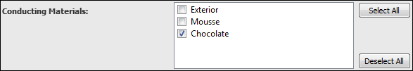
This port lists all the materials or labels contained in the connected Label Field. The user must select the heat conducting materials. If a material is not selected, it is considered as a thermal insulator with null thermal conductivity. By default, the material named Exterior or the value 0 is selected. At least one conducting material should be selected and all materials can be selected.

Thermal Flux Direction

This option allows the user to define the direction of the heat flux. Separate computations will be performed for each direction specified.

Spreadsheet

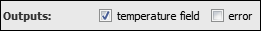
This port selects where the next result must appear. If "append result" is selected, the next result is appended in the connected spreadsheet to the last created table corresponding to the flow direction of this computation. If "new spreadsheet" is selected, the result is stored in a new spreadsheet. If no spreadsheet is connected, a new one is created. If the data connection has changed, results are automatically stored in a new spreadsheet in order to avoid any inconsistency in the Material thermal conductivity columns.

Outputs

If one of the check boxes is selected, the corresponding output will appear in the Project View at the end of the computation. The first check box stands for the resulting temperature field in the experimental setup. It is selected by default.

If the second checkbox is checked, a spreadsheet with suffix .TCExp.Error.Spreadsheet is added to the Project View. It contains the estimation of the error (or convergence criterion) at each iteration, for each computation (depending on how many directions are selected).

Note: the temperature field is automatically created as output of the module if the computation was aborted or did not converge. The created temperature field can be connected as an input of the module, so that the computed values can be used as initial solution of the problem (see above for more details).

Thermal Conductivity

This port is composed of a combo box and of a text field. The combo box contains all the materials or labels considered as heat conducting (that is to say selected in the Conducting Materials port). The content of the combo box is updated when the user changes the selection in the Conducting Materials port.

In the text field, the user can set the value of the thermal conductivity of the material currently selected in the combo box. The default value is 1 . If the thermal conductivity of a material is set to zero, the material will be considered as a thermal insulator.

Boundary Conditions

This port allows choosing the two boundary conditions to be imposed to the experimental system. The choices are "input temperature + output temperature", "input temperature + heat flux" and "output temperature + heat flux".

Note: thermal conductivity is independent from boundary conditions. Only the temperature field is rescaled according to boundary conditions.

Boundary Values

This port is updated depending on the pair of boundary conditions chosen in the Boundary Conditions port and lets the user set the values associated with these conditions.

Note: thermal conductivity is independent from boundary conditions. Only the temperature field is rescaled according to boundary values.

hxportgroup Advanced Settings

Advanced Settings

This port sets whether the additional options for fine tuning the module are visible (ON) or hidden (OFF). The options that appear when switching ON are considered to be expert options, which should not require any modification in most cases.

Refining Coefficient

Only appears when "show advanced settings" from port Options is checked. The refining coefficient can be used to artificially oversample an image, by simply dividing all the voxels by an integer value. This method gives better precision concerning the evaluation of the unknowns. It is an integer value, which must be strictly greater than 0. The slider is limited to 2 to avoid an accidental increase of this value, which would imply a heavy increase of unknown numbers, though a dramatic drop in computation time.

Relative Tolerance

Only appears when "show advanced settings" from port Options is checked. An iterative resolution with conjugate gradient and ILU preconditioner is used to solve Fourier equation system for the thermal conductivity computation (please refer to for more details). The convergence criterion used here is the relative decrease in the residual -norm. For convenience, the convergence criterion will often be simply called "error" in the GUI, spreadsheets and Console messages. Convergence is considered to be obtained at iteration if , where and is the linear system to solve. is the relative tolerance set in this port. It is a floating point value which must be greater than 0 and for which a default value of 10 is suggested.

Iterations

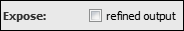
Only appears when "show advanced settings" from port Options is checked. The maximum number of iterations to compute is used to be sure that the computation loop will end even if the convergence criterion cannot be attained because of numerical approximation problems.

Expose

This checkbox stands for the refined image. The output that is shown in the Project View is the refined subvolume used for the computation. It means that the output field fits in the ROI if it is defined or has the same dimensions as the input data. It also means that the output field is oversampled by the factor indicated in the refining coefficient option.