Minimization with Gradient and Hessian Sparsity Pattern

This example shows how to solve a nonlinear minimization problem with tridiagonal Hessian matrix approximated by sparse finite differences instead of explicit computation.

The problem is to find x to minimize

$f (x) = \sum_{i = 1}^{n - 1} ({(x_{i}^{2})}^{(x_{i + 1}^{2} + 1)} + {(x_{i + 1}^{2})}^{(x_{i}^{2} + 1)}),$

where n = 1000.

To use the trust-region method in fminunc, you must compute the gradient in fun; it is not optional as in the quasi-newton method.

The brownfg file computes the objective function and gradient.

Step 1: Write a file brownfg.m that computes the objective function and the gradient of the objective.

This function file ships with your software.

function [f,g] = brownfg(x)
% BROWNFG Nonlinear minimization test problem
% 
% Evaluate the function
n=length(x); y=zeros(n,1);
i=1:(n-1);
y(i)=(x(i).^2).^(x(i+1).^2+1) + ...
        (x(i+1).^2).^(x(i).^2+1);
  f=sum(y);
% Evaluate the gradient if nargout > 1
  if nargout > 1
     i=1:(n-1); g = zeros(n,1);
     g(i) = 2*(x(i+1).^2+1).*x(i).* ...
              ((x(i).^2).^(x(i+1).^2))+ ...
              2*x(i).*((x(i+1).^2).^(x(i).^2+1)).* ...
              log(x(i+1).^2);
     g(i+1) = g(i+1) + ...
              2*x(i+1).*((x(i).^2).^(x(i+1).^2+1)).* ...
              log(x(i).^2) + ...
              2*(x(i).^2+1).*x(i+1).* ...
              ((x(i+1).^2).^(x(i).^2));
  end

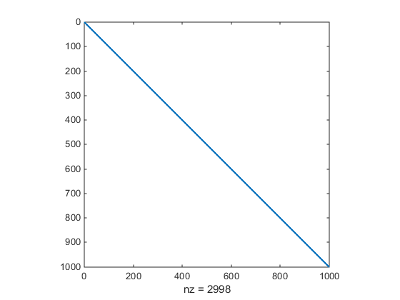
To allow efficient computation of the sparse finite-difference approximation of the Hessian matrix H(x), the sparsity structure of H must be predetermined. In this case assume this structure, Hstr, a sparse matrix, is available in file brownhstr.mat. Using the spy command you can see that Hstr is indeed sparse (only 2998 nonzeros). Use optimoptions to set the HessPattern option to Hstr. When a problem as large as this has obvious sparsity structure, not setting the HessPattern option requires a huge amount of unnecessary memory and computation because fminunc attempts to use finite differencing on a full Hessian matrix of one million nonzero entries.

You must also set the GradObj option to 'on' using optimoptions, since the gradient is computed in brownfg.m. Then execute fminunc as shown in Step 2.

Step 2: Call a nonlinear minimization routine with a starting point xstart.

fun = @brownfg;
load brownhstr % Get Hstr, structure of the Hessian
spy(Hstr) % View the sparsity structure of Hstr

n = 1000;
xstart = -ones(n,1); 
xstart(2:2:n,1) = 1;
options = optimoptions(@fminunc,'Algorithm','trust-region',...
    'GradObj','on','HessPattern',Hstr);
[x,fval,exitflag,output] = fminunc(fun,xstart,options);

This 1000-variable problem is solved in seven iterations and seven conjugate gradient iterations with a positive exitflag indicating convergence. The final function value and measure of optimality at the solution x are both close to zero (for fminunc, the first-order optimality is the infinity norm of the gradient of the function, which is zero at a local minimum):

exitflag,fval,output

exitflag =
     1

fval =
   7.4738e-17

output = 
         iterations: 7
          funcCount: 8
           stepsize: 0.0046
       cgiterations: 7
      firstorderopt: 7.9822e-10
          algorithm: 'trust-region'
            message: 'Local minimum found.…'
    constrviolation: []

Documentation