Set Up a Linear Program

Convert a Problem to Solver Form

This example shows how to convert a problem from mathematical form into Optimization Toolbox™ solver syntax. While the problem is a linear program, the techniques apply to all solvers.

The variables and expressions in the problem represent a model of operating a chemical plant, from an example in Edgar and Himmelblau [1]. There are two videos that describe the problem.

Optimization Modeling 1 Optimization Modeling 1 shows the problem in pictorial form. It shows how to generate the mathematical expressions of Model Description from the picture.
Optimization Modeling 2 Optimization Modeling 2 describes how to convert these mathematical expressions into Optimization Toolbox solver syntax. This video shows how to solve the problem, and how to interpret the results.

The remainder of this example is concerned solely with transforming the problem to solver syntax. The example closely follows the video Optimization Modeling 2 Optimization Modeling 2. The main difference between the video and the example is that this example shows how to use named variables, or index variables, which are similar to hash keys. This difference is in Combine Variables Into One Vector.

Model Description

The video Optimization Modeling 1 Optimization Modeling 1 suggests that one way to convert a problem into mathematical form is to:

Get an overall idea of the problem
Identify the goal (maximizing or minimizing something)
Identify (name) variables
Identify constraints
Determine which variables you can control
Specify all quantities in mathematical notation
Check the model for completeness and correctness

For the meaning of the variables in this section, see the video Optimization Modeling 1 Optimization Modeling 1.

The optimization problem is to minimize the objective function, subject to all the other expressions as constraints.

The objective function is:

0.002614 HPS + 0.0239 PP + 0.009825 EP.

The constraints are:

2500 ≤ P1 ≤ 6250
I1 ≤ 192,000
C ≤ 62,000
I1 - HE1 ≤ 132,000
I1 = LE1 + HE1 + C
1359.8 I1 = 1267.8 HE1 + 1251.4 LE1 + 192 C + 3413 P1
3000 ≤ P2 ≤ 9000
I2 ≤ 244,000
LE2 ≤ 142,000
I2 = LE2 + HE2
1359.8 I2 = 1267.8 HE2 + 1251.4 LE2 + 3413 P2
HPS = I1 + I2 + BF1
HPS = C + MPS + LPS
LPS = LE1 + LE2 + BF2
MPS = HE1 + HE2 + BF1 - BF2
P1 + P2 + PP ≥ 24,550
EP + PP ≥ 12,000
MPS ≥ 271,536
LPS ≥ 100,623
All variables are positive.

Solution Method

To solve the optimization problem, take the following steps.

Choose a Solver
Combine Variables Into One Vector
Write Bound Constraints
Write Linear Inequality Constraints
Write Linear Equality Constraints
Write the Objective
Solve the Problem with linprog
Examine the Solution

The steps are also shown in the video Optimization Modeling 2 Optimization Modeling 2.

Choose a Solver

To find the appropriate solver for this problem, consult the Optimization Decision Table. The table asks you to categorize your problem by type of objective function and types of constraints. For this problem, the objective function is linear, and the constraints are linear. The decision table recommends using the linprog solver.

As you see in Problems Handled by Optimization Toolbox Functions or the linprog function reference page, the linprog solver solves problems of the form

\min_{x} f^{T} x such that {\begin{matrix} A \cdot x \leq b, \\ A e q \cdot x = b e q, \\ l b \leq x \leq u b . \end{matrix}

(1-1)

f^Tx means a row vector of constants f multiplying a column vector of variables x. In other words,
f^Tx = f(1)x(1) + f(2)x(2) + ... + f(n)x(n),
where n is the length of f.
A x ≤ b represents linear inequalities. A is a k-by-n matrix, where k is the number of inequalities and n is the number of variables (size of x). b is a vector of length k. For more information, see Linear Inequality Constraints.
Aeq x = beq represents linear equalities. Aeq is an m-by-n matrix, where m is the number of equalities and n is the number of variables (size of x). beq is a vector of length m. For more information, see Linear Equality Constraints.
lb ≤ x ≤ ub means each element in the vector x must be greater than the corresponding element of lb, and must be smaller than the corresponding element of ub. For more information, see Bound Constraints.

The syntax of the linprog solver, as shown in its function reference page, is

[x fval] = linprog(f,A,b,Aeq,beq,lb,ub);

The inputs to the linprog solver are the matrices and vectors in Equation 1-1.

Combine Variables Into One Vector

There are 16 variables in the equations of Model Description. Put these variables into one vector. The name of the vector of variables is x in Equation 1-1. Decide on an order, and construct the components of x out of the variables.

The following code constructs the vector using a cell array of strings. Each string is the name of a variable.

variables = {'I1','I2','HE1','HE2','LE1','LE2','C','BF1',...
    'BF2','HPS','MPS','LPS','P1','P2','PP','EP'};
N = length(variables); 
% create variables for indexing 
for v = 1:N 
   eval([variables{v},' = ', num2str(v),';']); 
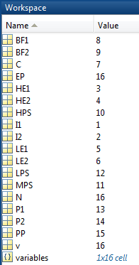
end

Executing these commands creates the following named variables in your workspace:

These named variables represent index numbers for the components of x. You do not have to create named variables. The video Optimization Modeling 2 Optimization Modeling 2 shows how to solve the problem simply using the index numbers of the components of x.

Write Bound Constraints

There are four variables with lower bounds, and six with upper bounds in the equations of Model Description. The lower bounds:

P1 ≥ 2500
P2 ≥ 3000
MPS ≥ 271,536
LPS ≥ 100,623.

Also, all the variables are positive, which means they have a lower bound of zero.

Create the lower bound vector lb as a vector of 0, then add the four other lower bounds.

lb = zeros(size(variables));
lb([P1,P2,MPS,LPS]) = ...
    [2500,3000,271536,100623];

The variables with upper bounds are:

P1 ≤ 6250
P2 ≤ 9000
I1 ≤ 192,000
I2 ≤ 244,000
C ≤ 62,000
LE2 ≤ 142000.

Create the upper bound vector as a vector of Inf, then add the six upper bounds.

ub = Inf(size(variables));
ub([P1,P2,I1,I2,C,LE2]) = ...
   [6250,9000,192000,244000,62000,142000];

Write Linear Inequality Constraints

There are three linear inequalities in the equations of Model Description:

I1 - HE1 ≤ 132,000
EP + PP ≥ 12,000
P1 + P2 + PP ≥ 24,550.

In order to have the equations in the form A x≤b, put all the variables on the left side of the inequality. All these equations already have that form. Ensure that each inequality is in "less than" form by multiplying through by –1 wherever appropriate:

I1 - HE1 ≤ 132,000
-EP - PP ≤ -12,000
-P1 - P2 - PP ≤ -24,550.

In your MATLAB^® workspace, create the A matrix as a 3-by-16 zero matrix, corresponding to 3 linear inequalities in 16 variables. Create the b vector with three components.

A = zeros(3,16);
A(1,I1) = 1; A(1,HE1) = -1; b(1) = 132000;
A(2,EP) = -1; A(2,PP) = -1; b(2) = -12000;
A(3,[P1,P2,PP]) = [-1,-1,-1];
b(3) = -24550;

Write Linear Equality Constraints

There are eight linear equations in the equations of Model Description:

I2 = LE2 + HE2
LPS = LE1 + LE2 + BF2
HPS = I1 + I2 + BF1
HPS = C + MPS + LPS
I1 = LE1 + HE1 + C
MPS = HE1 + HE2 + BF1 - BF2
1359.8 I1 = 1267.8 HE1 + 1251.4 LE1 + 192 C + 3413 P1
1359.8 I2 = 1267.8 HE2 + 1251.4 LE2 + 3413 P2.

In order to have the equations in the form Aeq x=beq, put all the variables on one side of the equation. The equations become:

LE2 + HE2 - I2 = 0
LE1 + LE2 + BF2 - LPS = 0
I1 + I2 + BF1 - HPS = 0
C + MPS + LPS - HPS = 0
LE1 + HE1 + C - I1 = 0
HE1 + HE2 + BF1 - BF2 - MPS = 0
1267.8 HE1 + 1251.4 LE1 + 192 C + 3413 P1 - 1359.8 I1 = 0
1267.8 HE2 + 1251.4 LE2 + 3413 P2 - 1359.8 I2 = 0.

Now write the Aeq matrix and beq vector corresponding to these equations. In your MATLAB workspace, create the Aeq matrix as an 8-by-16 zero matrix, corresponding to 8 linear equations in 16 variables. Create the beq vector with eight components, all zero.

Aeq = zeros(8,16); beq = zeros(8,1);
Aeq(1,[LE2,HE2,I2]) = [1,1,-1];
Aeq(2,[LE1,LE2,BF2,LPS]) = [1,1,1,-1];
Aeq(3,[I1,I2,BF1,HPS]) = [1,1,1,-1];
Aeq(4,[C,MPS,LPS,HPS]) = [1,1,1,-1];
Aeq(5,[LE1,HE1,C,I1]) = [1,1,1,-1];
Aeq(6,[HE1,HE2,BF1,BF2,MPS]) = [1,1,1,-1,-1];
Aeq(7,[HE1,LE1,C,P1,I1]) = [1267.8,1251.4,192,3413,-1359.8];
Aeq(8,[HE2,LE2,P2,I2]) = [1267.8,1251.4,3413,-1359.8];

Write the Objective

The objective function is

f^Tx = 0.002614 HPS + 0.0239 PP + 0.009825 EP.

Write this expression as a vector f of multipliers of the x vector:

f = zeros(size(variables));
f([HPS PP EP]) = [0.002614 0.0239 0.009825];

Solve the Problem with linprog

You now have inputs required by the linprog solver. Call the solver and print the outputs in formatted form:

[x fval] = linprog(f,A,b,Aeq,beq,lb,ub);
for d = 1:N
  fprintf('%12.2f \t%s\n',x(d),variables{d}) 
end
fval

The result:

Optimization terminated.
   136328.74 	I1
   244000.00 	I2
   128159.00 	HE1
   143377.00 	HE2
        0.00 	LE1
   100623.00 	LE2
     8169.74 	C
        0.00 	BF1
        0.00 	BF2
   380328.74 	HPS
   271536.00 	MPS
   100623.00 	LPS
     6250.00 	P1
     7060.71 	P2
    11239.29 	PP
      760.71 	EP

fval =
  1.2703e+003

Examine the Solution

The fval output gives the smallest value of the objective function at any feasible point.

The solution vector x is the point where the objective function has the smallest value. Notice that:

BF1, BF2, and LE1 are 0, their lower bounds.
I2 is 244,000, its upper bound.
The nonzero components of the f vector are
- HPS — 380,328.74
- PP — 11,239.29
- EP — 760.71

The video Optimization Modeling 2 Optimization Modeling 2 gives interpretations of these characteristics in terms of the original problem.

Bibliography

[1] Edgar, Thomas F., and David M. Himmelblau. Optimization of Chemical Processes. McGraw-Hill, New York, 1988.

Was this topic helpful?

Documentation