Documentation

Types of Constraints

Optimization Toolbox™ solvers have special forms for constraints:

• Bound Constraints — Lower and upper bounds on individual components: x ≥ l and x ≤ u.

• Linear Inequality Constraints — A·x ≤ b. A is an m-by-n matrix, which represents m constraints for an n-dimensional vector x. b is m-dimensional.

• Linear Equality Constraints — Aeq·x = beq. Equality constraints have the same form as inequality constraints.

• Nonlinear Constraints — c(x) ≤ 0 and ceq(x) = 0. Both c and ceq are scalars or vectors representing several constraints.

Optimization Toolbox functions assume that inequality constraints are of the form c_i(x) ≤ 0 or A x ≤ b. Express greater-than constraints as less-than constraints by multiplying them by –1. For example, a constraint of the form c_i(x) ≥ 0 is equivalent to the constraint –c_i(x) ≤ 0. A constraint of the form A·x ≥ b is equivalent to the constraint –A·x ≤ –b. For more information, see Linear Inequality Constraints and Nonlinear Constraints.

You can sometimes write constraints in several ways. For best results, use the lowest numbered constraints possible:

1. Bounds

2. Linear equalities

3. Linear inequalities

4. Nonlinear equalities

5. Nonlinear inequalities

For example, with a constraint 5 x ≤ 20, use a bound x ≤ 4 instead of a linear inequality or nonlinear inequality.

For information on how to pass extra parameters to constraint functions, see Passing Extra Parameters.

Iterations Can Violate Constraints

Be careful when writing your objective and constraint functions. Intermediate iterations can lead to points that are infeasible (do not satisfy constraints). If you write objective or constraint functions that assume feasibility, these functions can error or give unexpected results.

For example, if you take a square root or logarithm of x, and x < 0, the result is not real. You can try to avoid this error by setting 0 as a lower bound on x. Nevertheless, an intermediate iteration can violate this bound.

Algorithms That Satisfy Bound Constraints

Some solver algorithms satisfy bound constraints at every iteration:

• fmincon interior-point, sqp, and trust-region-reflective algorithms

• lsqcurvefit trust-region-reflective algorithm

• lsqnonlin trust-region-reflective algorithm

• fminbnd

Note:   If you set a lower bound equal to an upper bound, iterations can violate these constraints.

Solvers and Algorithms That Can Violate Bound Constraints

The following solvers and algorithms can violate bound constraints at intermediate iterations:

• fmincon active-set algorithm

• fgoalattain solver

• fminimax solver

• fseminf solver

Bound Constraints

Lower and upper bounds limit the components of the solution x.

If you know bounds on the location of an optimum, you can obtain faster and more reliable solutions by explicitly including these bounds in your problem formulation.

Give bounds as vectors with the same length as x, or as matrices with the same number of elements as x.

• If a particular component has no lower bound, use -Inf as the bound; similarly, use Inf if a component has no upper bound.

• If you have only bounds of one type (upper or lower), you do not need to write the other type. For example, if you have no upper bounds, you do not need to supply a vector of Infs.

• If only the first m out of n components have bounds, then you need only supply a vector of length m containing bounds. However, this shortcut causes solvers to throw a warning.

For example, suppose your bounds are:

x₃ ≥ 8
x₂ ≤ 3.

Write the constraint vectors as

l = [-Inf; -Inf; 8]
u = [Inf; 3] (throws a warning) or u = [Inf; 3; Inf].

Tip   Use Inf or -Inf instead of a large, arbitrary bound to lower memory usage and increase solver speed. See Use Inf Instead of a Large, Arbitrary Bound.

You need not give gradients for bound constraints; solvers calculate them automatically. Bounds do not affect Hessians.

For a more complex example of bounds, see Set Up a Linear Program.

Linear Inequality Constraints

Linear inequality constraints have the form A·x ≤ b. When A is m-by-n, there are m constraints on a variable x with n components. You supply the m-by-n matrix A and the m-component vector b.

Even if you pass an initial point x0 as a matrix, solvers pass the current point x as a column vector to linear constraints. See Matrix Arguments.

For example, suppose that you have the following linear inequalities as constraints:

x₁ + x₃ ≤ 4,
2x₂ – x₃ ≥ –2,
x₁ – x₂ + x₃ – x₄ ≥ 9.

Here m = 3 and n = 4.

Write these using the following matrix A and vector b:

$$\begin{array}{l}A=\left[\begin{array}{cccc}1& 0& 1& 0\\ 0& -2& 1& 0\\ -1& 1& -1& 1\end{array}\right],\\ b=\left[\begin{array}{c}4\\ 2\\ -9\end{array}\right].\end{array}$$

Notice that the "greater than" inequalities were first multiplied by –1 in order to get them into "less than" inequality form. In MATLAB^® syntax:

A = [1 0 1 0;
    0 -2 1 0;
    -1 1 -1 1];
b = [4;2;-9];

You do not need to give gradients for linear constraints; solvers calculate them automatically. Linear constraints do not affect Hessians.

For a more complex example of linear constraints, see Set Up a Linear Program.

Linear Equality Constraints

Linear equalities have the form Aeq·x = beq, which represents m equations with n-component vector x. You supply the m-by-n matrix Aeq and the m-component vector beq.

You do not need to give gradients for linear constraints; solvers calculate them automatically. Linear constraints do not affect Hessians. The form of this type of constraint is the same as for Linear Inequality Constraints.

Nonlinear Constraints

Nonlinear inequality constraints have the form c(x) ≤ 0, where c is a vector of constraints, one component for each constraint. Similarly, nonlinear equality constraints are of the form ceq(x) = 0.

Note:   Nonlinear constraint functions must return both c and ceq, the inequality and equality constraint functions, even if they do not both exist. Return empty [] for a nonexistent constraint.

For example, suppose that you have the following inequalities as constraints:

$$\begin{array}{c}\frac{x_1^2}{9}+\frac{x_2^2}{4}\le 1,\\ x_2\ge x_1^2-1.\end{array}$$

Write these constraints in a function file as follows:

function [c,ceq]=ellipseparabola(x)
c(1) = (x(1)^2)/9 + (x(2)^2)/4 - 1;
c(2) = x(1)^2 - x(2) - 1;
ceq = [];
end

Including Gradients in Constraint Functions

If you provide gradients for c and ceq, your solver can run faster and give more reliable results.

Providing a gradient has another advantage. A solver can reach a point x such that x is feasible, but finite differences around x always lead to an infeasible point. In this case, a solver can fail or halt prematurely. Providing a gradient allows a solver to proceed.

To include gradient information, write a conditionalized function as follows:

function [c,ceq,gradc,gradceq]=ellipseparabola(x)
c(1) = x(1)^2/9 + x(2)^2/4 - 1;
c(2) = x(1)^2 - x(2) - 1;
ceq = [];

if nargout > 2
    gradc = [2*x(1)/9, 2*x(1); ...
             x(2)/2, -1];
    gradceq = [];
end

See Writing Scalar Objective Functions for information on conditionalized functions. The gradient matrix has the form

gradc_{i, j} = [∂c(j)/∂x_i].

The first column of the gradient matrix is associated with c(1), and the second column is associated with c(2). This is the transpose of the form of Jacobians.

To have a solver use gradients of nonlinear constraints, indicate that they exist by using optimoptions:

options=optimoptions(@fmincon,'GradConstr','on');

Make sure to pass the options structure to your solver:

[x,fval] = fmincon(@myobj,x0,A,b,Aeq,beq,lb,ub, ...
           @ellipseparabola,options)

If you have a Symbolic Math Toolbox™ license, you can calculate gradients and Hessians automatically, as described in Symbolic Math Toolbox Calculates Gradients and Hessians.

Anonymous Nonlinear Constraint Functions

For information on anonymous objective functions, see Anonymous Function Objectives.

Nonlinear constraint functions must return two outputs. The first output corresponds to nonlinear inequalities, and the second corresponds to nonlinear equalities.

Anonymous functions return just one output. So how can you write an anonymous function as a nonlinear constraint?

The deal function distributes multiple outputs. For example, suppose your nonlinear inequalities are

$$\begin{array}{c}\frac{x_1^2}{9}+\frac{x_2^2}{4}\le 1,\\ x_2\ge x_1^2-1.\end{array}$$

Suppose that your nonlinear equality is

x₂ = tanh(x₁).

Write a nonlinear constraint function as follows:

c = @(x)[x(1)^2/9 + x(2)^2/4 - 1;
        x(1)^2 - x(2) - 1];
ceq = @(x)tanh(x(1)) - x(2);
nonlinfcn = @(x)deal(c(x),ceq(x));

To minimize the function cosh(x₁) + sinh(x₂) subject to the constraints in nonlinfcn, use fmincon:

obj = @(x)cosh(x(1))+sinh(x(2));
opts = optimoptions(@fmincon,'Algorithm','sqp');
z = fmincon(obj,[0;0],[],[],[],[],[],[],nonlinfcn,opts)

Local minimum found that satisfies the constraints.

Optimization completed because the objective function is 
non-decreasing in feasible directions, to within the default 
value of the function tolerance, and constraints are satisfied 
to within the default value of the constraint tolerance.

z =
   -0.6530
   -0.5737

To check how well the resulting point z satisfies the constraints, use nonlinfcn:

[cout,ceqout] = nonlinfcn(z)

cout =
   -0.8704
         0

ceqout =
     1.1102e-016

z indeed satisfies all the constraints to within the default value of the TolCon constraint tolerance, 1e-6.

Or Instead of And Constraints

In general, solvers takes constraints with an implicit AND:

constraint 1 AND constraint 2 AND constraint 3 are all satisfied.

However, sometimes you want an OR:

constraint 1 OR constraint 2 OR constraint 3 is satisfied.

These formulations are not logically equivalent, and there is generally no way to express OR constraints in terms of AND constraints.

Tip   Fortunately, nonlinear constraints are extremely flexible. You get OR constraints simply by setting the nonlinear constraint function to the minimum of the constraint functions.

The reason that you can set the minimum as the constraint is due to the nature of Nonlinear Constraints: you give them as a set of functions that must be negative at a feasible point. If your constraints are

F₁(x) ≤ 0 OR F₂(x) ≤ 0 OR F₃(x) ≤ 0,

then set the nonlinear inequality constraint function c(x) as:

c(x) = min(F₁(x),F₂(x),F₃(x)).

c(x) is not smooth, which is a general requirement for constraint functions, due to the minimum. Nevertheless, the method often works.

Note:   You cannot use the usual bounds and linear constraints in an OR constraint. Instead, convert your bounds and linear constraints to nonlinear constraint functions, as in this example.

For example, suppose your feasible region is the L-shaped region: x is in the rectangle –1 ≤ x(1) ≤ 1, 0 ≤ x(2) ≤ 1 OR x is in the rectangle 0 ≤ x(1) ≤ 1, –1 ≤ x(2) ≤ 1.

 Code for creating the figure

% Write the x and y coordinates of the figure, clockwise from (0,0)
x = [0,-1,-1,1,1,0,0];
y = [0,0,1,1,-1,-1,0];
plot(x,y)
xlim([-1.2 1.2])
ylim([-1.2 1.2])
axis equal

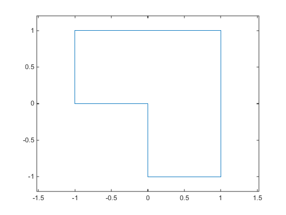
To represent a rectangle as a nonlinear constraint, instead of as bound constraints, construct a function that is negative inside the rectangle a ≤ x(1) ≤ b, c ≤ x(2) ≤ d:

function cout = rectconstr(x,a,b,c,d)
% Negative when  x is in the rectangle [a,b][c,d]
% First check that a,b,c,d are in the correct order

if (b <= a) || (d <= c)
    error('Give a rectangle a < b, c < d')
end

cout = max([(x(1)-b),(x(2)-d),(a-x(1)),(c-x(2))]);

Following the prescription of using the minimum of nonlinear constraint functions, for the L-shaped region, the nonlinear constraint function is:

function [c,ceq] = rectconstrfcn(x)

ceq = []; % no equality constraint
F(1) = rectconstr(x,-1,1,0,1); % one rectangle
F(2) = rectconstr(x,0,1,-1,1); % another rectangle
c = min(F); % for OR constraints

 Code for creating the figure

[xx,yy] = meshgrid(-2:.1:2);
x = [xx(:),yy(:)]; % one row per point

z = zeros(length(x),1); % allocate 
for ii = 1:length(x)
    [z(ii),~] = rectconstrfcn(x(ii,:));
end

z = reshape(z,size(xx));
surf(xx,yy,z)
colorbar
axis equal
xlabel('x');ylabel('y')
view(0,90)

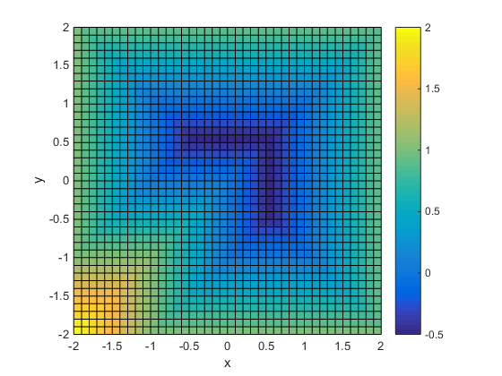
Suppose your objective function is

fun = @(x)exp(x(1)) * (4*x(1)^2 + 2*x(2)^2 + 4*x(1)*x(2) + 2*x(2) + 1);

Minimize fun over the L-shaped region:

opts = optimoptions(@fmincon,'Algorithm','interior-point','Display','off');
x0 = [-.5,.6]; % an arbitrary guess
[xsol,fval,eflag,output] = fmincon(fun,x0,[],[],[],[],[],[],@rectconstrfcn,opts)

xsol =

    0.4998   -0.9996


fval =

   2.4649e-07


eflag =

     1


output = 

         iterations: 17
          funcCount: 59
    constrviolation: 0
           stepsize: 1.8763e-04
          algorithm: 'interior-point'
      firstorderopt: 4.9302e-07
       cgiterations: 0
            message: 'Local minimum found that satisfies the constraints.…'

Clearly, the solution xsol is inside the L-shaped region. The exit flag is 1, indicating that xsol is a local minimum.

How to Use All Types of Constraints

This section contains an example of a nonlinear minimization problem with all possible types of constraints. The objective function is in the local function myobj(x). The nonlinear constraints are in the local function myconstr(x). This example does not use gradients.

function [x fval exitflag] = fullexample
x0 = [1; 4; 5; 2; 5];
lb = [-Inf; -Inf;  0; -Inf;   1];
ub = [ Inf;  Inf; 20; Inf; Inf];
Aeq = [1 -0.3 0 0 0];
beq = 0;
A = [0 0  0 -1  0.1
     0 0  0  1 -0.5
     0 0 -1  0  0.9];
b = [0; 0; 0];
opts = optimoptions(@fmincon,'Algorithm','sqp');
     
[x,fval,exitflag]=fmincon(@myobj,x0,A,b,Aeq,beq,lb,ub,...
                                  @myconstr,opts)

%---------------------------------------------------------
function f = myobj(x)

f = 6*x(2)*x(5) + 7*x(1)*x(3) + 3*x(2)^2;

%---------------------------------------------------------
function [c, ceq] = myconstr(x)

c = [x(1) - 0.2*x(2)*x(5) - 71
     0.9*x(3) - x(4)^2 - 67];
ceq = 3*x(2)^2*x(5) + 3*x(1)^2*x(3) - 20.875;

[x fval exitflag] = fullexample;

Local minimum found that satisfies the constraints.

Optimization completed because the objective function is non-decreasing in 
feasible directions, to within the default value of the function tolerance,
and constraints are satisfied to within the default value of the constraint tolerance.

x =
    0.6114
    2.0380
    1.3948
    0.1572
    1.5498

fval =
   37.3806

exitflag =
     1