Output Functions

What Is an Output Function?

For some problems, you might want output from an optimization algorithm at each iteration. For example, you might want to find the sequence of points that the algorithm computes and plot those points. To do this, create an output function that the optimization function calls at each iteration. See Output Function for details and syntax.

Generally, the solvers that can employ an output function are the ones that can take nonlinear functions as inputs. You can determine which solvers can have an output function by looking in the Options section of function reference pages, or by checking whether the Output function option is available in the Optimization app for a solver.

What the Example Contains

The following example continues the one in Nonlinear Inequality Constraints, which calls the function fmincon at the command line to solve a nonlinear, constrained optimization problem. The example in this section uses a function file to call fmincon. The file also contains all the functions needed for the example, including:

The objective function
The constraint function
An output function that records the history of points computed by the algorithm for fmincon. At each iteration of the algorithm for fmincon, the output function:
- Plots the current point computed by the algorithm.
- Stores the point and its corresponding objective function value in a variable called history, and stores the current search direction in a variable called searchdir. The search direction is a vector that points in the direction from the current point to the next one.

The code for the file is here: Writing the Example Function File.

Writing the Output Function

You specify the output function in options, such as

options = optimoptions(@fmincon,'OutputFcn',@outfun)

where outfun is the name of the output function. When you call an optimization function with options as an input, the optimization function calls outfun at each iteration of its algorithm.

In general, outfun can be any MATLAB^® function, but in this example, it is a nested function of the function file described in Writing the Example Function File. The following code defines the output function:

function stop = outfun(x,optimValues,state)
stop = false;
 
   switch state
       case 'init'
           hold on
       case 'iter'
           % Concatenate current point and objective function
           % value with history. x must be a row vector.
           history.fval = [history.fval; optimValues.fval];
           history.x = [history.x; x];
           % Concatenate current search direction with 
           % searchdir.
           searchdir = [searchdir;...
                        optimValues.searchdirection'];
           plot(x(1),x(2),'o');
           % Label points with iteration number.
           % Add .15 to x(1) to separate label from plotted 'o'
           text(x(1)+.15,x(2),num2str(optimValues.iteration));
       case 'done'
           hold off
       otherwise
   end
end

See Using Handles to Store Function Parameters in the MATLAB Programming Fundamentals documentation for more information about nested functions.

The arguments that the optimization function passes to outfun are:

x — The point computed by the algorithm at the current iteration
optimValues — Structure containing data from the current iteration
The example uses the following fields of optimValues:
- optimValues.iteration — Number of the current iteration
- optimValues.fval — Current objective function value
- optimValues.searchdirection — Current search direction
state — The current state of the algorithm ('init', 'interrupt', 'iter', or 'done')

For more information about these arguments, see Output Function.

Writing the Example Function File

To create the function file for this example:

Open a new file in the MATLAB Editor.

Copy and paste the following code into the file:

function [history,searchdir] = runfmincon
 
% Set up shared variables with OUTFUN
history.x = [];
history.fval = [];
searchdir = [];
 
% call optimization
x0 = [-1 1];
options = optimoptions(@fmincon,'OutputFcn',@outfun,... 
    'Display','iter','Algorithm','active-set');
xsol = fmincon(@objfun,x0,[],[],[],[],[],[],@confun,options);
 
 function stop = outfun(x,optimValues,state)
     stop = false;
 
     switch state
         case 'init'
             hold on
         case 'iter'
         % Concatenate current point and objective function
         % value with history. x must be a row vector.
           history.fval = [history.fval; optimValues.fval];
           history.x = [history.x; x];
         % Concatenate current search direction with 
         % searchdir.
           searchdir = [searchdir;... 
                        optimValues.searchdirection'];
           plot(x(1),x(2),'o');
         % Label points with iteration number and add title.
         % Add .15 to x(1) to separate label from plotted 'o'
           text(x(1)+.15,x(2),... 
                num2str(optimValues.iteration));
           title('Sequence of Points Computed by fmincon');
         case 'done'
             hold off
         otherwise
     end
 end
 
 function f = objfun(x)
     f = exp(x(1))*(4*x(1)^2 + 2*x(2)^2 + 4*x(1)*x(2) +... 
                    2*x(2) + 1);
 end
 
 function [c, ceq] = confun(x)
     % Nonlinear inequality constraints
     c = [1.5 + x(1)*x(2) - x(1) - x(2);
         -x(1)*x(2) - 10];
     % Nonlinear equality constraints
     ceq = [];
 end
end

Save the file as runfmincon.m in a folder on the MATLAB path.

Running the Example

To run the example, enter:

[history searchdir] = runfmincon;

This displays the following iterative output in the Command Window.

                                Max     Line search  Directional  First-order 
Iter F-count        f(x)   constraint   steplength   derivative   optimality Procedure 
   0      3       1.8394         0.5                                       Infeasible
   1      6      1.85127    -0.09197         1        0.109        0.778   start point
   2      9     0.300167        9.33         1       -0.117        0.313  Hessian modified 
   3     12     0.529835      0.9209         1         0.12        0.232   twice
   4     16     0.186965      -1.517       0.5       -0.224         0.13   
   5     19    0.0729085      0.3313         1       -0.121        0.054   
   6     22    0.0353323    -0.03303         1      -0.0542       0.0271   
   7     25    0.0235566    0.003184         1      -0.0271      0.00587   
   8     28    0.0235504  9.032e-008         1      -0.0146    8.51e-007   
Local minimum found that satisfies the constraints.

Optimization completed because the objective function is non-decreasing in 
feasible directions, to within the default value of the function tolerance,
and constraints are satisfied to within the default value of the constraint tolerance.

Active inequalities (to within options.TolCon = 1e-006):
  lower      upper     ineqlin   ineqnonlin
                                     1
                                     2

The output history is a structure that contains two fields:

history = 

       x: [9x2 double]
    fval: [9x1 double]

The fval field contains the objective function values corresponding to the sequence of points computed by fmincon:

history.fval

ans =

    1.8394
    1.8513
    0.3002
    0.5298
    0.1870
    0.0729
    0.0353
    0.0236
    0.0236

These are the same values displayed in the iterative output in the column with header f(x).

The x field of history contains the sequence of points computed by the algorithm:

history.x

ans =

   -1.0000    1.0000
   -1.3679    1.2500
   -5.5708    3.4699
   -4.8000    2.2752
   -6.7054    1.2618
   -8.0679    1.0186
   -9.0230    1.0532
   -9.5471    1.0471
   -9.5474    1.0474

This example displays a plot of this sequence of points, in which each point is labeled by its iteration number.

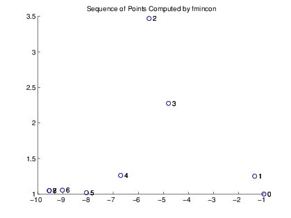
The optimal point occurs at the eighth iteration. Note that the last two points in the sequence are so close that they overlap.

The second output argument, searchdir, contains the search directions for fmincon at each iteration. The search direction is a vector pointing from the point computed at the current iteration to the point computed at the next iteration:

searchdir =

   -0.3679    0.2500
   -4.2029    2.2199
    0.7708   -1.1947
   -3.8108   -2.0268
   -1.3625   -0.2432
   -0.9552    0.0346
   -0.5241   -0.0061
   -0.0003    0.0003

Was this topic helpful?

Documentation