Documentation

Plot an Optimization During Execution

You can plot various measures of progress during the execution of a solver. Set the PlotFcns name-value pair in optimoptions, and specify one or more plotting functions for the solver to call at each iteration. Pass a function handle or cell array of function handles.

There are a variety of predefined plot functions available. See:

• The PlotFcns option description in the solver function reference page

• Optimization app > Options > Plot functions

You can also use a custom-written plot function. Write a function file using the same structure as an output function. For more information on this structure, see Output Function.

Using a Plot Function

This example shows how to use a plot function to view the progress of the fmincon interior-point algorithm. The problem is taken from the Getting Started Solve a Constrained Nonlinear Problem. The first part of the example shows how to run the optimization using the Optimization app. The second part shows how to run the optimization from the command line.

Note:   The Optimization app warns that it will be removed in a future release.

Running the Optimization Using the Optimization App

1. Write the nonlinear objective and constraint functions, including the derivatives:

   function [f g H] = rosenboth(x)
   % ROSENBOTH returns both the value y of Rosenbrock's function
   % and also the value g of its gradient and H the Hessian.
   
   f = 100*(x(2) - x(1)^2)^2 + (1-x(1))^2;
   
   if nargout > 1
       g = [-400*(x(2)-x(1)^2)*x(1)-2*(1-x(1));
           200*(x(2)-x(1)^2)];
       
       if nargout > 2
           H = [1200*x(1)^2-400*x(2)+2, -400*x(1);
               -400*x(1), 200];  
       end
   end

   Save this file as rosenboth.m.

   function [c,ceq,gc,gceq] = unitdisk2(x)
   % UNITDISK2 returns the value of the constraint
   % function for the disk of radius 1 centered at
   % [0 0]. It also returns the gradient.
   
   c = x(1)^2 + x(2)^2 - 1;
   ceq = [ ];
   
   if nargout > 2
       gc = [2*x(1);2*x(2)];
       gceq = [];
   end

   Save this file as unitdisk2.m.

2. Start the Optimization app by entering optimtool at the command line.

3. Set up the optimization:

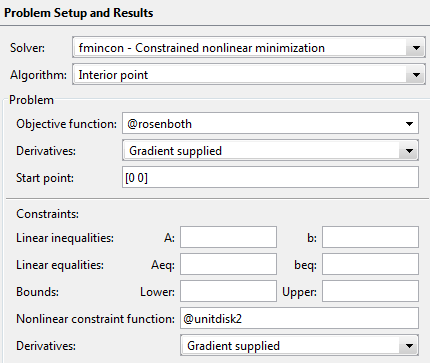
   • Choose the fmincon solver.

   • Choose the Interior point algorithm.

   • Set the objective function to @rosenboth.

   • Choose Gradient supplied for the objective function derivative.

   • Set the start point to [0 0].

   • Set the nonlinear constraint function to @unitdisk2.

   • Choose Gradient supplied for the nonlinear constraint derivatives.

   Your Problem Setup and Results panel should match the following figure.

   

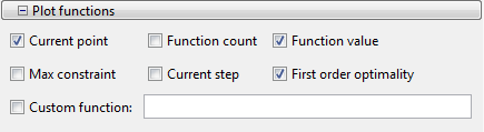
4. Choose three plot functions in the Options pane: Current point, Function value, and First order optimality.

   

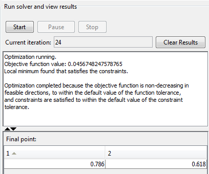
5. Click the Start button under Run solver and view results.

6. The output appears as follows in the Optimization app.

   

   In addition, the following three plots appear in a separate window.

   

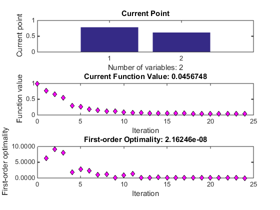
• The "Current Point" plot graphically shows the minimizer [0.786,0.618], which is reported as the Final point in the Run solver and view results pane. This plot updates at each iteration, showing the intermediate iterates.

• The "Current Function Value" plot shows the objective function value at all iterations. This graph is nearly monotone, showing fmincon reduces the objective function at almost every iteration.

• The "First-order Optimality" plot shows the first-order optimality measure at all iterations.

Running the Optimization from the Command Line

1. Write the nonlinear objective and constraint functions, including the derivatives, as shown in Running the Optimization Using the Optimization App.

2. Create an options structure that includes calling the three plot functions:

   options = optimoptions(@fmincon,'Algorithm','interior-point',...
    'GradObj','on','GradConstr','on','PlotFcns',{@optimplotx,...
       @optimplotfval,@optimplotfirstorderopt});

3. Call fmincon:

   x = fmincon(@rosenboth,[0 0],[],[],[],[],[],[],...
       @unitdisk2,options)

4. fmincon gives the following output:

   Local minimum found that satisfies the constraints.
   
   Optimization completed because the objective function is
   non-decreasing in feasible directions, to within the default
   value of the function tolerance, and constraints are satisfied
   to within the default value of the constraint tolerance.
   
   x =
       0.7864    0.6177

   fmincon also displays the three plot functions, shown at the end of Running the Optimization Using the Optimization App.