Solve a Constrained Nonlinear Problem

Problem Formulation: Rosenbrock's Function

Consider the problem of minimizing Rosenbrock's function

$f (x) = 100 {(x_{2} - x_{1}^{2})}^{2} + {(1 - x_{1})}^{2},$

over the unit disk, i.e., the disk of radius 1 centered at the origin. In other words, find x that minimizes the function f(x) over the set $x_{1}^{2} + x_{2}^{2} \leq 1$ . This problem is a minimization of a nonlinear function with a nonlinear constraint.

Note: Rosenbrock's function is a standard test function in optimization. It has a unique minimum value of 0 attained at the point (1,1). Finding the minimum is a challenge for some algorithms since it has a shallow minimum inside a deeply curved valley.

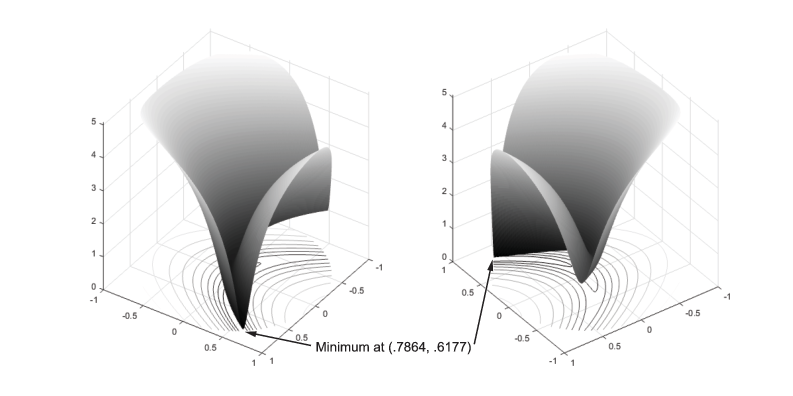
Here are two views of Rosenbrock's function in the unit disk. The vertical axis is log-scaled; in other words, the plot shows log(1+f(x)). Contour lines lie beneath the surface plot.

Rosenbrock's function, log-scaled: two views.

Code for generating the figure

function createfigure

% Create figure
figure1 = figure('Position',[1 400 1200 600]);
colormap('gray');
axis square;
R=0:.002:1;
TH=2*pi*(0:.002:1); 
X=R'*cos(TH); 
Y=R'*sin(TH); 
Z=log(1+vrosenbrock(X,Y));

% Create subplot
subplot1 = subplot(1,2,1,'Parent',figure1);
view([124 34]);
grid('on');
hold('all');

% Create surface
surf(X,Y,Z,'Parent',subplot1,'LineStyle','none');

% Create contour
contour(X,Y,Z,'Parent',subplot1);

% Create subplot
subplot2 = subplot(1,2,2,'Parent',figure1);
view([234 34]);
grid('on');
hold('all');

% Create surface
surf(X,Y,Z,'Parent',subplot2,'LineStyle','none');

% Create contour
contour(X,Y,Z,'Parent',subplot2);

The function vrosenbrock, used in createfigure, calculates Rosenbrock's function at a whole vector of points:

function z=vrosenbrock(x,y)

z=100*(y - x.^2).^2 + (1-x).^2;

The function f(x) is called the objective function. This is the function you wish to minimize. The inequality $x_{1}^{2} + x_{2}^{2} \leq 1$ is called a constraint. Constraints limit the set of x over which you may search for a minimum. You can have any number of constraints, which are inequalities or equations.

All Optimization Toolbox™ optimization functions minimize an objective function. To maximize a function f, apply an optimization routine to minimize –f. For more details about maximizing, see Maximizing an Objective.

Defining the Problem in Toolbox Syntax

To use Optimization Toolbox software, you need to

Define your objective function in the MATLAB^® language, as a function file or anonymous function. This example will use a function file.
Define your constraint(s) as a separate file or anonymous function.

Function File for Objective Function

A function file is a text file containing MATLAB commands with the extension .m. Create a new function file in any text editor, or use the built-in MATLAB Editor as follows:

At the command line enter:
```
edit rosenbrock
```
The MATLAB Editor opens.

In the editor enter:

function f = rosenbrock(x)
f = 100*(x(2) - x(1)^2)^2 + (1 - x(1))^2;

Save the file by selecting File > Save.

File for Constraint Function

Constraint functions must be formulated so that they are in the form c(x) ≤ 0 or ceq(x) = 0. The constraint $x_{1}^{2} + x_{2}^{2} \leq 1$ needs to be reformulated as $x_{1}^{2} + x_{2}^{2} - 1 \leq 0$ in order to have the correct syntax.

Furthermore, toolbox functions that accept nonlinear constraints need to have both equality and inequality constraints defined. In this example there is only an inequality constraint, so you must pass an empty array [] as the equality constraint function ceq.

With these considerations in mind, write a function file for the nonlinear constraint:

Create a file named unitdisk.m containing the following code:

function [c, ceq] = unitdisk(x)
c = x(1)^2 + x(2)^2 - 1;
ceq = [ ];

Save the file unitdisk.m.

Running the Optimization

There are two ways to run the optimization:

Using the Optimization app
Using command line functions; see Minimizing at the Command Line.

Optimization app

Note: The Optimization app warns that it will be removed in a future release.

Start the Optimization app by typing optimtool at the command line.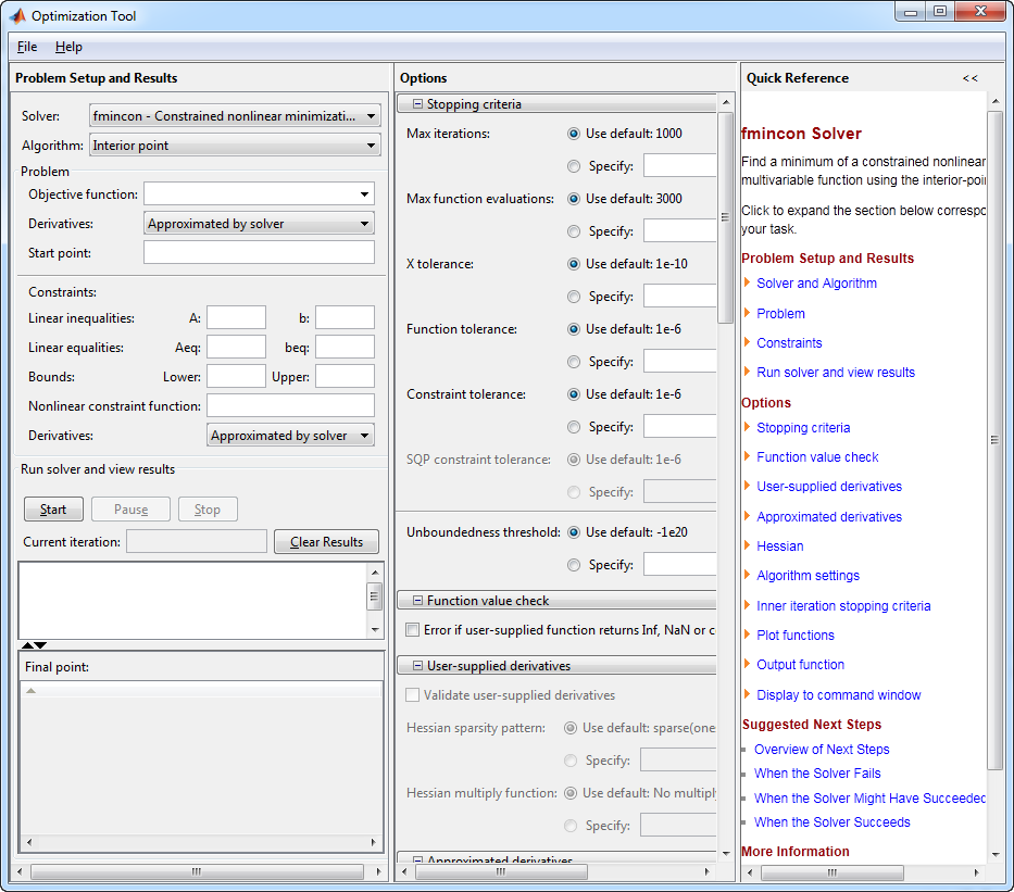

For more information about this tool, see Optimization App.
The default Solver fmincon - Constrained nonlinear minimization is selected. This solver is appropriate for this problem, since Rosenbrock's function is nonlinear, and the problem has a constraint. For more information about how to choose a solver, see Choosing a Solver.
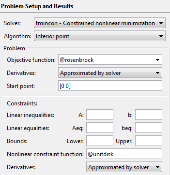
In the Algorithm pop-up menu choose Interior point, which is the default.
For Objective function enter @rosenbrock. The @ character indicates that this is a function handle of the file rosenbrock.m.
For Start point enter [0 0]. This is the initial point where fmincon begins its search for a minimum.
For Nonlinear constraint function enter @unitdisk, the function handle of unitdisk.m.
Your Problem Setup and Results pane should match this figure.
In the Options pane (center bottom), select iterative in the Level of display pop-up menu. (If you don't see the option, click Display to command window.) This shows the progress of fmincon in the command window.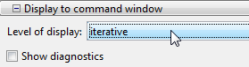
Click Start under Run solver and view results.

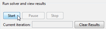
The following message appears in the box below the Start button:

Optimization running.
Objective function value: 0.045674824758137236
Local minimum found that satisfies the constraints.

Optimization completed because the objective function is non-decreasing in 
feasible directions, to within the default value of the function tolerance,
and constraints are satisfied to within the default value of the constraint tolerance.

Your objective function value may differ slightly, depending on your computer system and version of Optimization Toolbox software.

The message tells you that:

The search for a constrained optimum ended because the derivative of the objective function is nearly 0 in directions allowed by the constraint.
The constraint is satisfied to the requisite accuracy.

Exit Flags and Exit Messages discusses exit messages such as these.

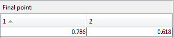
The minimizer x appears under Final point.

Minimizing at the Command Line

You can run the same optimization from the command line, as follows.

Create an options structure to choose iterative display and the interior-point algorithm:

options = optimoptions(@fmincon,...
    'Display','iter','Algorithm','interior-point');

Run the fmincon solver with the options structure, reporting both the location x of the minimizer, and value fval attained by the objective function:
```
[x,fval] = fmincon(@rosenbrock,[0 0],...
    [],[],[],[],[],[],@unitdisk,options)
```
The six sets of empty brackets represent optional constraints that are not being used in this example. See the fmincon function reference pages for the syntax.

MATLAB outputs a table of iterations, and the results of the optimization:

Local minimum found that satisfies the constraints.

Optimization completed because the objective function is non-decreasing in 
feasible directions, to within the selected value of the function tolerance,
and constraints are satisfied to within the selected value of the constraint tolerance.

x =
    0.7864    0.6177

fval =
    0.0457

The message tells you that the search for a constrained optimum ended because the derivative of the objective function is nearly 0 in directions allowed by the constraint, and that the constraint is satisfied to the requisite accuracy. Several phrases in the message contain links that give you more information about the terms used in the message. For more details about these links, see Enhanced Exit Messages.

Interpreting the Result

The iteration table in the command window shows how MATLAB searched for the minimum value of Rosenbrock's function in the unit disk. This table is the same whether you use Optimization app or the command line. MATLAB reports the minimization as follows:

                                            First-order      Norm of
 Iter F-count            f(x)  Feasibility   optimality         step
    0       3    1.000000e+00    0.000e+00    2.000e+00
    1      13    7.753537e-01    0.000e+00    6.250e+00    1.768e-01
    2      18    6.519648e-01    0.000e+00    9.048e+00    1.679e-01
    3      21    5.543209e-01    0.000e+00    8.033e+00    1.203e-01
    4      24    2.985207e-01    0.000e+00    1.790e+00    9.328e-02
    5      27    2.653799e-01    0.000e+00    2.788e+00    5.723e-02
    6      30    1.897216e-01    0.000e+00    2.311e+00    1.147e-01
    7      33    1.513701e-01    0.000e+00    9.706e-01    5.764e-02
    8      36    1.153330e-01    0.000e+00    1.127e+00    8.169e-02
    9      39    1.198058e-01    0.000e+00    1.000e-01    1.522e-02
   10      42    8.910052e-02    0.000e+00    8.378e-01    8.301e-02
   11      45    6.771960e-02    0.000e+00    1.365e+00    7.149e-02
   12      48    6.437664e-02    0.000e+00    1.146e-01    5.701e-03
   13      51    6.329037e-02    0.000e+00    1.883e-02    3.774e-03
   14      54    5.161934e-02    0.000e+00    3.016e-01    4.464e-02
   15      57    4.964194e-02    0.000e+00    7.913e-02    7.894e-03
   16      60    4.955404e-02    0.000e+00    5.462e-03    4.185e-04
   17      63    4.954839e-02    0.000e+00    3.993e-03    2.208e-05
   18      66    4.658289e-02    0.000e+00    1.318e-02    1.255e-02
   19      69    4.647011e-02    0.000e+00    8.006e-04    4.940e-04
   20      72    4.569141e-02    0.000e+00    3.136e-03    3.379e-03
   21      75    4.568281e-02    0.000e+00    6.439e-05    3.974e-05
   22      78    4.568281e-02    0.000e+00    8.000e-06    1.083e-07
   23      81    4.567641e-02    0.000e+00    1.601e-06    2.793e-05
   24      84    4.567482e-02    0.000e+00    2.062e-08    6.916e-06

This table might differ from yours depending on toolbox version and computing platform. The following description applies to the table as displayed.

The first column, labeled Iter, is the iteration number from 0 to 24. fmincon took 24 iterations to converge.
The second column, labeled F-count, reports the cumulative number of times Rosenbrock's function was evaluated. The final row shows an F-count of 84, indicating that fmincon evaluated Rosenbrock's function 84 times in the process of finding a minimum.
The third column, labeled f(x), displays the value of the objective function. The final value, 0.04567482, is the minimum that is reported in the Optimization app Run solver and view results box, and at the end of the exit message in the command window.
The fourth column, Feasibility, is 0 for all iterations. This column shows the value of the constraint function unitdisk at each iteration where the constraint is positive. Since the value of unitdisk was negative in all iterations, every iteration satisfied the constraint.

The other columns of the iteration table are described in Iterative Display.

Was this topic helpful?

Documentation