Optimization App
Note: The Optimization app warns that it will be removed in a future release. |
Optimization App Basics
How to Open the Optimization App
To open the Optimization app, type
optimtool
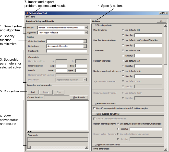
in the Command Window. This opens the Optimization app, as shown in the following figure.

You can also start the Optimization app from the MATLAB® Apps tab.

The reference page for the Optimization app provides variations
for starting the optimtool function.
Examples that Use the Optimization App
The following documentation examples use the optimization app:
Steps for Using the Optimization App
This is a summary of the steps to set up your optimization problem and view results with the Optimization app.
Pausing and Stopping
While a solver is running, you can
Click Pause to temporarily suspend the algorithm. To resume the algorithm using the current iteration at the time you paused, click Resume.
Click Stop to stop the algorithm. The Run solver and view results window displays information for the current iteration at the moment you clicked Stop.
You can export your results after stopping the algorithm. For details, see Exporting Your Work.
Viewing Results
When a solver terminates, the Run solver and view results window displays the reason the algorithm terminated. To clear the Run solver and view results window between runs, click Clear Results.
Sorting the Displayed Results. Depending on the solver and problem, results can be in the form of a table. If the table has multiple rows, sort the table by clicking a column heading. Click the heading again to sort the results in reverse.
For example, suppose you use the Optimization app to solve the lsqlin problem
described in Optimization App with the lsqlin Solver. The result appears
as follows.
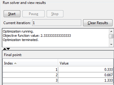
To sort the results by value, from lowest to highest, click Value. The results were already in that order, so don't change.
To sort the results in reverse order, highest to lowest, click Value again.
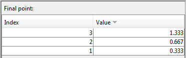
To return to the original order, click Index.
For an example of sorting a table returned by the Global Optimization Toolbox gamultiobj function,
see Multiobjective Optimization with Two Objectives.
If you export results using File > Export to Workspace, the exported results do not depend on the sorted display.
Final Point
The Final point updates to show the coordinates
of the final point when the algorithm terminated. If you don't see
the final point, click the upward-pointing triangle on the
![]() icon on the lower-left.
icon on the lower-left.
Starting a New Problem
Resetting Options and Clearing the Problem. Selecting File > Reset Optimization Tool resets the problem definition and options to the original default values. This action is equivalent to closing and restarting the app.
To clear only the problem definition, select File > Clear Problem Fields. With this action, fields in the Problem Setup and Results pane are reset to the defaults, with the exception of the selected solver and algorithm choice. Any options that you have modified from the default values in the Options pane are not reset with this action.
Setting Preferences for Changing Solvers. To modify how your options are handled in the Optimization app when you change solvers, select File > Preferences, which opens the Preferences dialog box shown below.
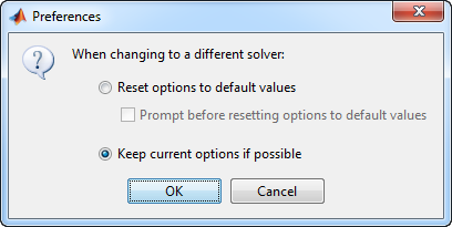
The default value, Reset options to defaults,
discards any options you specified previously in the optimtool.
Under this choice, you can select the option Prompt before
resetting options to defaults.
Alternatively, you can select Keep current options if possible to preserve the values you have modified. Changed options that are not valid with the newly selected solver are kept but not used, while active options relevant to the new solver selected are used. This choice allows you to try different solvers with your problem without losing your options.
Specifying Certain Options
Plot Functions
You can select a plot function to easily plot various measures of progress while the algorithm executes. Each plot selected draws a separate axis in the figure window. If available for the solver selected, the Stop button in the Run solver and view results window to interrupt a running solver. You can select a predefined plot function from the Optimization app, or you can select Custom function to write your own. Plot functions not relevant to the solver selected are grayed out. The following lists the available plot functions:
Current point — Select to show a bar plot of the point at the current iteration.
Function count — Select to plot the number of function evaluations at each iteration.
Function value — Select to plot the function value at each iteration.
Norm of residuals — Select to show a bar plot of the current norm of residuals at the current iteration.
Max constraint — Select to plot the maximum constraint violation value at each iteration.
Current step — Select to plot the algorithm step size at each iteration.
First order optimality — Select to plot the violation of the optimality conditions for the solver at each iteration.
Custom function — Enter your own plot function as a function handle. To provide more than one plot function use a cell array, for example, by typing:
Write custom plot functions with the same syntax as output functions. For information, see Output Function.{@plotfcn,@plotfcn2}
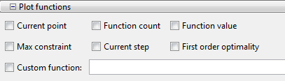
The graphic above shows the plot functions available for the
default fmincon solver.
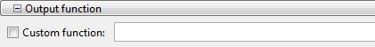
Output function
Output function is a function or collection of functions the algorithm calls at each iteration. Through an output function you can observe optimization quantities such as function values, gradient values, and current iteration. Specify no output function, a single output function using a function handle, or multiple output functions. To provide more than one output function use a cell array of function handles in the Custom function field, for example by typing:
{@outputfcn,@outputfcn2}For more information on writing an output function, see Output Function.
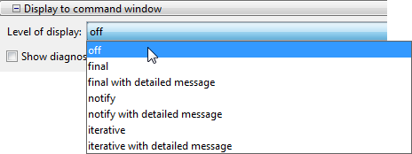
Display to Command Window
Select Level of display to specify the amount of information displayed when you run the algorithm. Choose from the following; depending on the solver, only some may be available:
off(default) — Display no output.final— Display the reason for stopping at the end of the run.final with detailed message— Display the detailed reason for stopping at the end of the run.notify— Display output only if the function does not converge.notify with detailed message— Display a detailed output only if the function does not converge.iterative— Display information at each iteration of the algorithm and the reason for stopping at the end of the run.iterative with detailed message— Display information at each iteration of the algorithm and the detailed reason for stopping at the end of the run.
See Enhanced Exit Messages for information on detailed messages.
Selecting Show diagnostics lists problem information and options that have changed from the defaults.
The graphic below shows the display options for the fmincon solver.
Some other solvers have fewer options.
Importing and Exporting Your Work
Exporting Your Work
The Export to Workspace dialog box enables you to send your problem information to the MATLAB workspace as a structure or object that you may then manipulate in the Command Window.
To access the Export to Workspace dialog box shown below, select File > Export to Workspace.
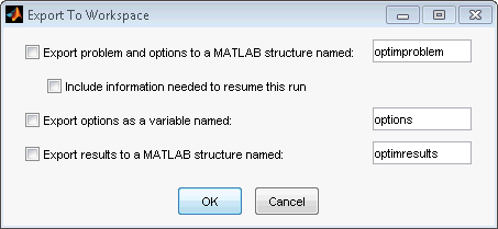
You can specify results that contain:
The problem and options information
The problem and options information, and the state of the solver when stopped (this means the latest point for most solvers, the current population for Genetic Algorithms solvers, and the best point found for the Simulated Annealing solver)
The states of random number generators
randandrandnat the start of the previous run, by checking the Use random states from previous run box for applicable solversThe options information only
The results of running your problem in the Optimization app
Exported results contain all optional information.
For example, an exported results structure for lsqcurvefit contains
the data x, resnorm, residual, exitflag, output, lambda,
and jacobian.
After you have exported information from the Optimization app
to the MATLAB workspace, you can see your data in the MATLAB Workspace
browser or by typing the name of the structure at the Command Window.
To see the value of a field in a structure or object, double-click
the name in the Workspace window. Alternatively, see the values by
entering exportname.fieldname at the command line.
For example, so see the message in an output structure, enter output.message.
If a structure contains structures or objects, you can double-click
again in the workspace browser, or enter exportname.name2.fieldname at
the command line. For example, to see the level of iterative display
contained in the options of an exported problem structure, enter optimproblem.options.Display.
You can run a solver on an exported problem at the command line by typing
solver(problem)
fmincon problem named optimproblem,
you can typefmincon(optimproblem)
fmincon on the problem with the saved options
in optimproblem. You can exercise more control
over outputs by typing, for example,[x,fval,exitflag] = fmincon(optimproblem)
Importing Your Work
Whether you save options from Optimization Toolbox™ functions at the Command Window, or whether you export options, or the problem and options, from the Optimization app, you can resume work on your problem using the Optimization app.
There are three ways to import your options, or problem and options, to the Optimization app:
Call the
optimtoolfunction from the Command Window specifying your options, or problem and options, as the input, for example,optimtool(options)
Select File > Import Options in the Optimization app.
Select File > Import Problem in the Optimization app.
The methods described above require that the options, or problem and options, be present in the MATLAB workspace.
If you import a problem that was generated with the Include information needed to resume this run box checked, the initial point is the latest point generated in the previous run. (For Genetic Algorithm solvers, the initial population is the latest population generated in the previous run. For the Simulated Annealing solver, the initial point is the best point generated in the previous run.) If you import a problem that was generated with this box unchecked, the initial point (or population) is the initial point (or population) of the previous run.
Generating a File
You may want to generate a file to continue with your optimization problem in the Command Window at another time. You can run the file without modification to recreate the results that you created with the Optimization app. You can also edit and modify the file and run it from the Command Window.
To export data from the Optimization app to a file, select File > Generate Code.
The generated file captures the following:
The problem definition, including the solver, information on the function to be minimized, algorithm specification, constraints, and start point
The options with the currently selected option value
Running the file at the Command Window reproduces your problem results.
Although you cannot export your problem results to a generated file, you can save them in a MAT-file that you can use with your generated file, by exporting the results using the Export to Workspace dialog box, then saving the data to a MAT-file from the Command Window.