Documentation

What Can Be Wrong If The Solver Succeeds?

A solver can report that a minimization succeeded, and yet the reported solution can be incorrect. For a rather trivial example, consider minimizing the function f(x) = x³ for x between –2 and 2, starting from the point 1/3:

options = optimoptions('fmincon','Algorithm','active-set');
ffun = @(x)x^3;
xfinal = fmincon(ffun,1/3,[],[],[],[],-2,2,[],options)         

Local minimum found that satisfies the constraints.

Optimization completed because the objective function is
non-decreasing in feasible directions, to within the default  
valueof the function tolerance, and constraints were satisfied 
to within the default value of the constraint tolerance.

No active inequalities.

xfinal =
 -1.5056e-008

The true minimum occurs at x = -2. fmincon gives this report because the function f(x) is so flat near x = 0.

Another common problem is that a solver finds a local minimum, but you might want a global minimum. For more information, see Local vs. Global Optima.

Lesson: check your results, even if the solver reports that it "found" a local minimum, or "solved" an equation.

This section gives techniques for verifying results.

1. Change the Initial Point

The initial point can have a large effect on the solution. If you obtain the same or worse solutions from various initial points, you become more confident in your solution.

For example, minimize f(x) = x³ + x⁴ starting from the point 1/4:

ffun = @(x)x^3 + x^4;
options = optimoptions('fminunc','Algorithm','quasi-newton');
[xfinal fval] = fminunc(ffun,1/4,options)

Local minimum found.

Optimization completed because the size of the gradient 
is less than the default value of the function tolerance.

x =
 -1.6764e-008

fval =
 -4.7111e-024

Change the initial point by a small amount, and the solver finds a better solution:

[xfinal fval] = fminunc(ffun,1/4+.001,options)

Local minimum found.

Optimization completed because the size of the gradient 
is less than the default value of the function tolerance.

xfinal =
   -0.7500

fval =
   -0.1055

x = -0.75 is the global solution; starting from other points cannot improve the solution.

For more information, see Local vs. Global Optima.

2. Check Nearby Points

To see if there are better values than a reported solution, evaluate your objective function and constraints at various nearby points.

For example, with the objective function ffun from What Can Be Wrong If The Solver Succeeds?, and the final point xfinal = -1.5056e-008, calculate ffun(xfinal±Δ) for some Δ:

delta = .1;
[ffun(xfinal),ffun(xfinal+delta),ffun(xfinal-delta)]

ans =
   -0.0000    0.0011   -0.0009

The objective function is lower at ffun(xfinal-Δ), so the solver reported an incorrect solution.

A less trivial example:

options = optimoptions(@fmincon,'Algorithm','active-set');
lb = [0,-1]; ub = [1,1];
ffun = @(x)(x(1)-(x(1)-x(2))^2);
[x fval exitflag] = fmincon(ffun,[1/2 1/3],[],[],[],[],...
                           lb,ub,[],options)

Local minimum found that satisfies the constraints.

Optimization completed because the objective function is
non-decreasing in feasible directions, to within the default  
valueof the function tolerance, and constraints were satisfied 
to within the default value of the constraint tolerance.

Active inequalities (to within options.TolCon = 1e-006):
  lower      upper     ineqlin   ineqnonlin
    1                                 

x =
  1.0e-007 *
         0    0.1614

fval =
 -2.6059e-016

exitflag =
     1

Evaluating ffun at nearby feasible points shows that the solution x is not a true minimum:

[ffun([0,.001]),ffun([0,-.001]),...
    ffun([.001,-.001]),ffun([.001,.001])]

ans =
  1.0e-003 *
   -0.0010   -0.0010    0.9960    1.0000

The first two listed values are smaller than the computed minimum fval.

If you have a Global Optimization Toolbox license, you can use the patternsearch function to check nearby points.

3. Check your Objective and Constraint Functions

Double-check your objective function and constraint functions to ensure that they correspond to the problem you intend to solve. Suggestions:

• Check the evaluation of your objective function at a few points.

• Check that each inequality constraint has the correct sign.

• If you performed a maximization, remember to take the negative of the reported solution. (This advice assumes that you maximized a function by minimizing the negative of the objective.) For example, to maximize f(x) = x – x², minimize g(x) = –x + x²:

  options = optimoptions('fminunc','Algorithm','quasi-newton');
  [x fval] = fminunc(@(x)-x+x^2,0,options)
  
  Local minimum found.
  
  Optimization completed because the size of the gradient is 
  less than the default value of the function tolerance.
  
  x =
      0.5000
  
  fval =
     -0.2500

  The maximum of f is 0.25, the negative of fval.

• Check that an infeasible point does not cause an error in your functions; see Iterations Can Violate Constraints.

Local vs. Global Optima

• Why Didn't the Solver Find the Smallest Minimum?

• Searching for a Smaller Minimum

• Basins of Attraction

Why Didn't the Solver Find the Smallest Minimum?

In general, solvers return a local minimum. The result might be a global minimum, but there is no guarantee that it is. This section describes why solvers behave this way, and gives suggestions for ways to search for a global minimum, if needed.

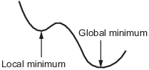
• A local minimum of a function is a point where the function value is smaller than at nearby points, but possibly greater than at a distant point.

• A global minimum is a point where the function value is smaller than at all other feasible points.

Generally, Optimization Toolbox™ solvers find a local optimum. (This local optimum can be a global optimum.) They find the optimum in the basin of attraction of the starting point. For more information about basins of attraction, see Basins of Attraction.

There are some exceptions to this general rule.

• Linear programming and positive definite quadratic programming problems are convex, with convex feasible regions, so there is only one basin of attraction. Indeed, under certain choices of options, linprog ignores any user-supplied starting point, and quadprog does not require one, though supplying one can sometimes speed a minimization.

• Global Optimization Toolbox functions, such as simulannealbnd, attempt to search more than one basin of attraction.

Searching for a Smaller Minimum

If you need a global optimum, you must find an initial value for your solver in the basin of attraction of a global optimum.

Suggestions for ways to set initial values to search for a global optimum:

• Use a regular grid of initial points.

• Use random points drawn from a uniform distribution if your problem has all its coordinates bounded. Use points drawn from normal, exponential, or other random distributions if some components are unbounded. The less you know about the location of the global optimum, the more spread-out your random distribution should be. For example, normal distributions rarely sample more than three standard deviations away from their means, but a Cauchy distribution (density 1/(π(1 + x²))) makes hugely disparate samples.

• Use identical initial points with added random perturbations on each coordinate, bounded, normal, exponential, or other.

• If you have a Global Optimization Toolbox license, use the GlobalSearch or MultiStart solvers. These solvers automatically generate random start points within bounds.

The more you know about possible initial points, the more focused and successful your search will be.

Basins of Attraction

If an objective function f(x) is smooth, the vector –∇f(x) points in the direction where f(x) decreases most quickly. The equation of steepest descent, namely

$$\frac{d}{dt}x(t)=-\nabla f(x(t)),$$

yields a path x(t) that goes to a local minimum as t gets large. Generally, initial values x(0) that are near to each other give steepest descent paths that tend to the same minimum point. The basin of attraction for steepest descent is the set of initial values that lead to the same local minimum.

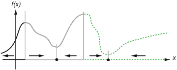
The following figure shows two one-dimensional minima. The figure shows different basins of attraction with different line styles, and shows directions of steepest descent with arrows. For this and subsequent figures, black dots represent local minima. Every steepest descent path, starting at a point x(0), goes to the black dot in the basin containing x(0).

One-dimensional basins

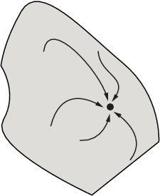
The following figure shows how steepest descent paths can be more complicated in more dimensions.

One basin of attraction, showing steepest descent paths from various starting points

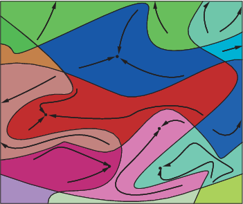
The following figure shows even more complicated paths and basins of attraction.

Several basins of attraction

Constraints can break up one basin of attraction into several pieces. For example, consider minimizing y subject to:

• y ≥ |x|

• y ≥ 5 – 4(x–2)².

The figure shows the two basins of attraction with the final points.

 Code for Generating the Figure

syms x y
myabs = abs(x);
mycurve = 5 - 4*(x-2)^2;
myline = feval(symengine,'max',myabs,mycurve);
mybrdr = 1 + heaviside(x-2);
myarea = heaviside(y - myline)*mybrdr;
% myarea = 0 where infeasible, 1 when x < 2, 2 when x > 2
marinv = 1/myarea; % removes the infeasible region

plot(0,0,'k.','MarkerSize',25);
hold on
plot(11/4,11/4,'k.','MarkerSize',25);
ezplot(mycurve,[.9 3])
ezplot(myabs,[-2 5])
ezsurf(marinv,[-2,5,-1,6],500)

The steepest descent paths are straight lines down to the constraint boundaries. From the constraint boundaries, the steepest descent paths travel down along the boundaries. The final point is either (0,0) or (11/4,11/4), depending on whether the initial x-value is above or below 2.