Root of nonlinear function
Calculate
by finding the zero of the sine function near 3.
fun = @sin; % function x0 = 3; % initial point x = fzero(fun,x0)
x =
3.1416
Find the zero of cosine between 1 and 2.
fun = @cos; % function x0 = [1 2]; % initial interval x = fzero(fun,x0)
x =
1.5708
Note that cos(1) and cos(2) differ in sign.
Find a zero of the function f(x) = x3 – 2x – 5.
First, write a file called f.m.
function y = f(x)
y = x.^3-2*x-5;Save f.m on your MATLAB® path.
Find the zero of f(x)
near 2.
fun = @f; % function x0 = 2; % initial point z = fzero(fun,x0)
z =
2.0946Since f(x) is a polynomial, you can
find the same real zero, and a complex conjugate pair of zeros, using
the roots command.
roots([1 0 -2 -5])
ans = 2.0946 -1.0473 + 1.1359i -1.0473 - 1.1359i
Find the root of a function that has an extra parameter.
myfun = @(x,c) cos(c*x); % parameterized function c = 2; % parameter fun = @(x) myfun(x,c); % function of x alone x = fzero(fun,0.1)
x =
0.7854
Plot the solution process by setting some plot functions.
Define the function and initial point.
fun = @(x)sin(cosh(x)); x0 = 1;
Examine the solution process by setting options that include plot functions.
options = optimset('PlotFcns',{@optimplotx,@optimplotfval});
Run fzero including options.
x = fzero(fun,x0,options)
x =
1.8115

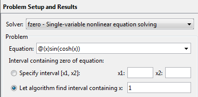
Solve a problem that is defined by an export from Optimization app.
Define a problem in Optimization app. Enter optimtool('fzero'),
and fill in the problem as pictured.
Note: The Optimization app warns that it will be removed in a future release. |

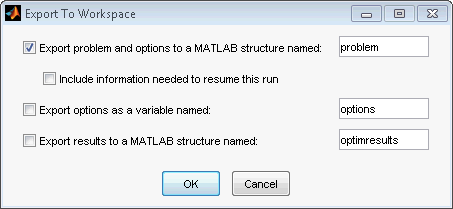
Select File > Export to Workspace,
and export the problem as pictured to a variable named problem.

Enter the following at the command line.
x = fzero(problem)
x =
1.8115Find the point where exp(-exp(-x)) = x, and display information about the solution process.
fun = @(x) exp(-exp(-x)) - x; % function x0 = [0,1]; % initial interval options = optimset('Display','iter'); % show iterations [x,fval,exitflag,output] = fzero(fun,x0,options)
Func-count x f(x) Procedure
2 1 -0.307799 initial
3 0.544459 0.0153522 interpolation
4 0.566101 0.00070708 interpolation
5 0.567143 -1.40255e-08 interpolation
6 0.567143 1.50013e-12 interpolation
7 0.567143 0 interpolation
Zero found in the interval [0, 1]
x =
0.5671
fval =
0
exitflag =
1
output =
intervaliterations: 0
iterations: 5
funcCount: 7
algorithm: 'bisection, interpolation'
message: 'Zero found in the interval [0, 1]'
fval = 0 means fun(x) = 0, as desired.
fun — Function to solvefunction handleFunction to solve, specified as a handle to a scalar-valued
function. fun accepts a scalar x and
returns a scalar fun(x).
fzero solves fun(x) = 0. To solve an equation fun(x) = c(x),
instead solve fun2(x) = fun(x) - c(x) = 0.
To include extra parameters in your function, see the example Root of Function with Extra Parameter and the section Passing Extra Parameters.
Example: @sin
Example: @myFunction
Example: @(x)(x-a)^5 - 3*x + a - 1
Data Types: function_handle
x0 — Initial valuescalar | 2-element vectorInitial value, specified as a real scalar or a 2-element real vector.
Scalar — fzero begins at x0 and
tries to locate a point x1 where fun(x1) has
the opposite sign of fun(x0). Then fzero iteratively
shrinks the interval where fun changes sign to
reach a solution.
2-element vector — fzero checks
that fun(x0(1)) and fun(x0(2)) have
opposite signs, and errors if they do not. It then iteratively shrinks
the interval where fun changes sign to reach a
solution. An interval x0 must be finite; it cannot
contain ±Inf.
Tip
Calling |
Example: 3
Example: [2,17]
Data Types: double
options — Options for solution processstructure, typically created using optimsetOptions for solution process, specified as a structure. Create
or modify the options structure using optimset. fzero uses
these options structure fields.
| Level of display (see Iterative Display):
|
| Check whether objective function values are valid.
|
| Specify one or more user-defined
functions that an optimization function calls at each iteration, either
as a function handle or as a cell array of function handles. The default
is none ( |
| Plot various measures of progress
while the algorithm executes. Select from predefined plots or write
your own. Pass a function handle or a cell array of function handles.
The default is none (
For information on writing a custom plot function, see Plot Functions. |
| Termination tolerance on |
Example: options = optimset('FunValCheck','on')
Data Types: struct
problem — Root-finding problemstructureRoot-finding problem, specified as a structure with all of the following fields.
| Objective function |
| Initial point for x,
scalar or 2-D vector |
| 'fzero' |
| Options structure, typically created
using optimset |
You can generate problem by exporting from
Optimization app. See Importing and Exporting Your Work or Solve Exported Problem.
Data Types: struct
x — Location of root or sign changereal scalarLocation of root or sign change, returned as a scalar.
fval — Function value at xreal scalarFunction value at x, returned as a scalar.
exitflag — Integer encoding the exit conditionintegerInteger encoding the exit condition, meaning the reason fzero stopped
its iterations.
| Function converged to a solution |
| Algorithm was terminated by the output function or plot function. |
|
|
-4 | Complex function value was encountered while searching for an interval containing a sign change. |
-5 | Algorithm might have converged to a singular point. |
-6 |
|
output — Information about root-finding processstructureInformation about root-finding process, returned as a structure. The fields of the structure are:
intervaliterations | Number of iterations taken to find an interval containing a root |
iterations | Number of zero-finding iterations |
funcCount | Number of function evaluations |
algorithm |
|
message | Exit message |
[1] Brent, R., Algorithms for Minimization Without Derivatives, Prentice-Hall, 1973.
[2] Forsythe, G. E., M. A. Malcolm, and C. B. Moler, Computer Methods for Mathematical Computations, Prentice-Hall, 1976.