fsolve

Solve system of nonlinear equations

Nonlinear system solver

Solves a problem specified by

F(x) = 0

for x, where F(x) is a function that returns a vector value.

x is a vector or a matrix; see Matrix Arguments.

Syntax

  • x = fsolve(fun,x0)
    example
  • x = fsolve(fun,x0,options)
    example
  • x = fsolve(problem)
    example
  • [x,fval] = fsolve(___)
    example
  • [x,fval,exitflag,output] = fsolve(___)
    example
  • [x,fval,exitflag,output,jacobian] = fsolve(___)

Description

example

x = fsolve(fun,x0) starts at x0 and tries to solve the equations fun(x) = 0, an array of zeros.

example

x = fsolve(fun,x0,options) solves the equations with the optimization options specified in options. Use optimoptions to set these options.

example

x = fsolve(problem) solves problem, where problem is a structure described in Input Arguments. Create the problem structure by exporting a problem from Optimization app, as described in Exporting Your Work.

example

[x,fval] = fsolve(___), for any syntax, returns the value of the objective function fun at the solution x.

example

[x,fval,exitflag,output] = fsolve(___) additionally returns a value exitflag that describes the exit condition of fsolve, and a structure output with information about the optimization process.

[x,fval,exitflag,output,jacobian] = fsolve(___) returns the Jacobian of fun at the solution x.

Examples

collapse all

Solution of 2-D Nonlinear System

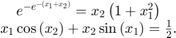
This example shows how to solve two nonlinear equations in two variables. The equations are

$$ \begin{array}{c}
{e^{ - {e^{ - ({x_1} + {x_2})}}}} = {x_2}\left( {1 + x_1^2} \right)\\
{x_1}\cos \left( {{x_2}} \right) + {x_2}\sin \left( {{x_1}} \right) = \frac{1}{2}.
\end{array} $$

Convert the equations to the form $F(x) = \bf{0}$.

$$\begin{array}{c}
{e^{ - {e^{ - ({x_1} + {x_2})}}}} - {x_2}\left( {1 + x_1^2} \right) = 0\\
{x_1}\cos \left( {{x_2}} \right) + {x_2}\sin \left( {{x_1}} \right)
- \frac{1}{2} = 0. \end{array} $$

Write a function that computes the left-hand side of these two equations.


% Copyright 2015 The MathWorks, Inc.

function F = root2d(x)

F(1) = exp(-exp(-x(1)+x(2))) - x(2)*(1+x(1)^2);
F(2) = x(1)*cos(x(2)) + x(2)*sin(x(1)) - 0.5;

Save this code as a file named root2d.m on your MATLAB® path.

Solve the system of equations starting at the point [0,0].

fun = @root2d;
x0 = [0,0];
x = fsolve(fun,x0)
Equation solved.

fsolve completed because the vector of function values is near zero
as measured by the default value of the function tolerance, and
the problem appears regular as measured by the gradient.


x =

    0.3931    0.3366

Solution with Nondefault Options

Examine the solution process for a nonlinear system.

Set options to have no display and a plot function that displays the first-order optimality, which should converge to 0 as the algorithm iterates.

options = optimoptions('fsolve','Display','none','PlotFcns',@optimplotfirstorderopt);

The equations in the nonlinear system are

$$\begin{array}{c}
{e^{ - {e^{ - ({x_1} + {x_2})}}}} = {x_2}\left( {1 + x_1^2} \right)\\
{x_1}\cos \left( {{x_2}} \right) + {x_2}\sin \left( {{x_1}} \right) = \frac{1}{2}.
\end{array} $$

Convert the equations to the form $F(x) = \bf{0}$.

$$\begin{array}{c}
{e^{ - {e^{ - ({x_1} + {x_2})}}}} - {x_2}\left( {1 + x_1^2} \right) = 0\\
{x_1}\cos \left( {{x_2}} \right) + {x_2}\sin \left( {{x_1}} \right)
- \frac{1}{2} = 0. \end{array} $$

Write a function that computes the left-hand side of these two equations.


% Copyright 2015 The MathWorks, Inc.

function F = root2d(x)

F(1) = exp(-exp(-x(1)+x(2))) - x(2)*(1+x(1)^2);
F(2) = x(1)*cos(x(2)) + x(2)*sin(x(1)) - 0.5;

Save this code as a file named root2d.m on your MATLAB® path.

Solve the nonlinear system starting from the point [0,0] and observe the solution process.

fun = @root2d;
x0 = [0,0];
x = fsolve(fun,x0,options)
x =

    0.3931    0.3366

Solve a Problem Structure

Create a problem structure for fsolve and solve the problem.

Solve the same problem as in Solution with Nondefault Options, but formulate the problem using a problem structure.

Set options for the problem to have no display and a plot function that displays the first-order optimality, which should converge to 0 as the algorithm iterates.

problem.options = optimoptions('fsolve','Display','none','PlotFcns',@optimplotfirstorderopt);

The equations in the nonlinear system are

$$\begin{array}{c}
{e^{ - {e^{ - ({x_1} + {x_2})}}}} = {x_2}\left( {1 + x_1^2} \right)\\
{x_1}\cos \left( {{x_2}} \right) + {x_2}\sin \left( {{x_1}} \right) = \frac{1}{2}.
\end{array} $$

Convert the equations to the form $F(x) = \bf{0}$.

$$\begin{array}{c}
{e^{ - {e^{ - ({x_1} + {x_2})}}}} - {x_2}\left( {1 + x_1^2} \right) = 0\\
{x_1}\cos \left( {{x_2}} \right) + {x_2}\sin \left( {{x_1}} \right)
- \frac{1}{2} = 0. \end{array} $$

Write a function that computes the left-hand side of these two equations.


% Copyright 2015 The MathWorks, Inc.

function F = root2d(x)

F(1) = exp(-exp(-x(1)+x(2))) - x(2)*(1+x(1)^2);
F(2) = x(1)*cos(x(2)) + x(2)*sin(x(1)) - 0.5;

Save this code as a file named root2d.m on your MATLAB® path.

Create the remaining fields in the problem structure.

problem.objective = @root2d;
problem.x0 = [0,0];
problem.solver = 'fsolve';

Solve the problem.

x = fsolve(problem)
x =

    0.3931    0.3366

Solution Process of Nonlinear System

This example returns the iterative display showing the solution process for the system of two equations and two unknowns

2x1x2=ex1x1+2x2=ex2.

Rewrite the equations in the form F(x) = 0:

2x1x2ex1=0x1+2x2ex2=0.

Start your search for a solution at x0 = [-5 -5].

First, write a file that computes F, the values of the equations at x.

function F = myfun(x)
F = [2*x(1) - x(2) - exp(-x(1));
      -x(1) + 2*x(2) - exp(-x(2))];

Save this function file as myfun.m on your MATLAB® path.

Set up the initial point. Set options to return iterative display.

x0 = [-5;-5];
options = optimoptions('fsolve','Display','iter');

Call fsolve.

[x,fval] = fsolve(@myfun,x0,options)
                                  Norm of  First-order Trust-region
Iteration Func-count    f(x)        step   optimality       radius
    0        3       23535.6                2.29e+004        1
    1        6       6001.72           1    5.75e+003        1
    2        9       1573.51           1    1.47e+003        1
    3       12       427.226           1          388        1
    4       15       119.763           1          107        1
    5       18       33.5206           1         30.8        1
    6       21       8.35208           1         9.05        1
    7       24       1.21394           1         2.26        1
    8       27      0.016329    0.759511        0.206      2.5
    9       30  3.51575e-006    0.111927      0.00294      2.5
   10       33  1.64763e-013  0.00169132    6.36e-007      2.5

Equation solved.

fsolve completed because the vector of function values is near zero
as measured by the default value of the function tolerance, and
the problem appears regular as measured by the gradient.

x =
    0.5671
    0.5671

fval =
  1.0e-006 *
      -0.4059
      -0.4059

Examine Matrix Equation Solution

Find a matrix X that satisfies

X*X*X=[1234],

starting at the point x= [1,1;1,1]. Examine the fsolve outputs to see the solution quality and process.

Create an anonymous function that calculates the matrix equation.

fun = @(x)x*x*x - [1,2;3,4];

Set options to turn off the display. Set the initial point x0.

options = optimoptions('fsolve','Display','off');
x0 = ones(2);

Call fsolve and obtain information about the solution process.

[x,fval,exitflag,output] = fsolve(fun,x0,options)
x =

   -0.1291    0.8602
    1.2903    1.1612


fval =

   1.0e-09 *

   -0.1621    0.0780
    0.1167   -0.0465


exitflag =

     1


output = 

       iterations: 6
        funcCount: 35
        algorithm: 'trust-region-dogleg'
    firstorderopt: 2.4488e-10
          message: 'Equation solved.

fsolve completed because the vector of function...'

The exit flag value 1 indicates that the solution is reliable. To verify this manually, calculate the residual (sum of squares of fval) to see how close it is to zero.

sum(sum(Fval.*Fval))
ans = 
   4.8133e-20

This small residual confirms that x is a solution.

fsolve performed 35 function evaluations to find the solution, as you can see in the output structure.

output.funcCount
ans =

    35

Related Examples

Input Arguments

collapse all

fun — Nonlinear equations to solvefunction handle | function name

Nonlinear equations to solve, specified as a function handle or function name. fun is a function that accepts a vector x and returns a vector F, the nonlinear equations evaluated at x. The equations to solve are F = 0 for all components of F. The function fun can be specified as a function handle for a file

x = fsolve(@myfun,x0)

where myfun is a MATLAB function such as

function F = myfun(x)
F = ...            % Compute function values at x

fun can also be a function handle for an anonymous function.

x = fsolve(@(x)sin(x.*x),x0);

If the user-defined values for x and F are matrices, they are converted to a vector using linear indexing.

If the Jacobian can also be computed and the Jacobian option is 'on', set by

options = optimoptions('fsolve','Jacobian','on')

the function fun must return, in a second output argument, the Jacobian value J, a matrix, at x.

If fun returns a vector (matrix) of m components and x has length n, where n is the length of x0, the Jacobian J is an m-by-n matrix where J(i,j) is the partial derivative of F(i) with respect to x(j). (The Jacobian J is the transpose of the gradient of F.)

Example: fun = @(x)x*x*x-[1,2;3,4]

Data Types: char | function_handle

x0 — Initial pointreal vector | real array

Initial point, specified as a real vector or real array. fsolve uses the number of elements in and size of x0 to determine the number and size of variables that fun accepts.

Example: x0 = [1,2,3,4]

Data Types: double

options — Optimization optionsoutput of optimoptions | structure as optimset returns

Optimization options, specified as the output of optimoptions or a structure as optimset returns.

Some options apply to all algorithms, and others are relevant for particular algorithms. See Optimization Options Reference for detailed information.

All Algorithms

Algorithm

Choose between 'trust-region-dogleg' (default), 'trust-region-reflective', and 'levenberg-marquardt'. Set the initial Levenberg-Marquardt parameter λ by setting Algorithm to a cell array such as {'levenberg-marquardt',.005}. The default λ = 0.01.

The Algorithm option specifies a preference for which algorithm to use. It is only a preference because for the trust-region-reflective algorithm, the nonlinear system of equations cannot be underdetermined; that is, the number of equations (the number of elements of F returned by fun) must be at least as many as the length of x. Similarly, for the trust-region-dogleg algorithm, the number of equations must be the same as the length of x. fsolve uses the Levenberg-Marquardt algorithm when the selected algorithm is unavailable. For more information on choosing the algorithm, see Choosing the Algorithm.

DerivativeCheck

Compare user-supplied derivatives (gradients of objective or constraints) to finite-differencing derivatives. The choices are 'on' or the default 'off'.

Diagnostics

Display diagnostic information about the function to be minimized or solved. The choices are 'on' or the default 'off'.

DiffMaxChange

Maximum change in variables for finite-difference gradients (a positive scalar). The default is Inf.

DiffMinChange

Minimum change in variables for finite-difference gradients (a positive scalar). The default is 0.

Display

Level of display (see Iterative Display):

  • 'off' or 'none' displays no output.

  • 'iter' displays output at each iteration, and gives the default exit message.

  • 'iter-detailed' displays output at each iteration, and gives the technical exit message.

  • 'final' (default) displays just the final output, and gives the default exit message.

  • 'final-detailed' displays just the final output, and gives the technical exit message.

FinDiffRelStep

Scalar or vector step size factor for finite differences. When you set FinDiffRelStep to a vector v, forward finite differences steps delta are

delta = v.*sign′(x).*max(abs(x),TypicalX);

where sign′(x) = sign(x) except sign′(0) = 1. Central finite differences are

delta = v.*max(abs(x),TypicalX);

Scalar FinDiffRelStep expands to a vector. The default is sqrt(eps) for forward finite differences, and eps^(1/3) for central finite differences.

FinDiffType

Finite differences, used to estimate gradients, are either 'forward' (default), or 'central' (centered). 'central' takes twice as many function evaluations, but should be more accurate.

The algorithm is careful to obey bounds when estimating both types of finite differences. So, for example, it could take a backward, rather than a forward, difference to avoid evaluating at a point outside bounds.

FunValCheck

Check whether objective function values are valid. 'on' displays an error when the objective function returns a value that is complex, Inf, or NaN. The default, 'off', displays no error.

Jacobian

If 'on', fsolve uses a user-defined Jacobian (defined in fun), or Jacobian information (when using JacobMult), for the objective function. If 'off' (default), fsolve approximates the Jacobian using finite differences.

MaxFunEvals

Maximum number of function evaluations allowed, a positive integer. The default is 100*numberOfVariables. See Tolerances and Stopping Criteria and Iterations and Function Counts.

MaxIter

Maximum number of iterations allowed, a positive integer. The default is 400. See Tolerances and Stopping Criteria and Iterations and Function Counts.

OutputFcn

Specify one or more user-defined functions that an optimization function calls at each iteration, either as a function handle or as a cell array of function handles. The default is none ([]). See Output Function.

PlotFcns

Plots various measures of progress while the algorithm executes. Select from predefined plots or write your own. Pass a function handle or a cell array of function handles. The default is none ([]):

  • @optimplotx plots the current point.

  • @optimplotfunccount plots the function count.

  • @optimplotfval plots the function value.

  • @optimplotstepsize plots the step size.

  • @optimplotfirstorderopt plots the first-order optimality measure.

For information on writing a custom plot function, see Plot Functions.

TolFun

Termination tolerance on the function value, a positive scalar. The default is 1e-6. See Tolerances and Stopping Criteria.

TolX

Termination tolerance on x, a positive scalar. The default is 1e-6. See Tolerances and Stopping Criteria.

TypicalX

Typical x values. The number of elements in TypicalX is equal to the number of elements in x0, the starting point. The default value is ones(numberofvariables,1). fsolve uses TypicalX for scaling finite differences for gradient estimation.

The trust-region-dogleg algorithm uses TypicalX as the diagonal terms of a scaling matrix.

Trust-Region-Reflective Algorithm

JacobMult

Function handle for Jacobian multiply function. For large-scale structured problems, this function computes the Jacobian matrix product J*Y, J'*Y, or J'*(J*Y) without actually forming J. The function is of the form

W = jmfun(Jinfo,Y,flag)

where Jinfo contains a matrix used to compute J*Y (or J'*Y, or J'*(J*Y)). The first argument Jinfo must be the same as the second argument returned by the objective function fun, for example, in

[F,Jinfo] = fun(x)

Y is a matrix that has the same number of rows as there are dimensions in the problem. flag determines which product to compute:

  • If flag == 0, W = J'*(J*Y).

  • If flag > 0, W = J*Y.

  • If flag < 0, W = J'*Y.

In each case, J is not formed explicitly. fsolve uses Jinfo to compute the preconditioner. See Passing Extra Parameters for information on how to supply values for any additional parameters jmfun needs.

    Note   'Jacobian' must be set to 'on' for fsolve to pass Jinfo from fun to jmfun.

See Minimization with Dense Structured Hessian, Linear Equalities for a similar example.


JacobPattern

Sparsity pattern of the Jacobian for finite differencing. Set JacobPattern(i,j) = 1 when fun(i) depends on x(j). Otherwise, set JacobPattern(i,j) = 0. In other words, JacobPattern(i,j) = 1 when you can have ∂fun(i)/∂x(j) ≠ 0.

Use JacobPattern when it is inconvenient to compute the Jacobian matrix J in fun, though you can determine (say, by inspection) when fun(i) depends on x(j). fsolve can approximate J via sparse finite differences when you give JacobPattern.

In the worst case, if the structure is unknown, do not set JacobPattern. The default behavior is as if JacobPattern is a dense matrix of ones. Then fsolve computes a full finite-difference approximation in each iteration. This can be very expensive for large problems, so it is usually better to determine the sparsity structure.


MaxPCGIter

Maximum number of PCG (preconditioned conjugate gradient) iterations, a positive scalar. The default is max(1,floor(numberOfVariables/2)). For more information, see Equation Solving Algorithms.


PrecondBandWidth

Upper bandwidth of preconditioner for PCG, a nonnegative integer. The default PrecondBandWidth is Inf, which means a direct factorization (Cholesky) is used rather than the conjugate gradients (CG). The direct factorization is computationally more expensive than CG, but produces a better quality step towards the solution. Set PrecondBandWidth to 0 for diagonal preconditioning (upper bandwidth of 0). For some problems, an intermediate bandwidth reduces the number of PCG iterations.


TolPCG

Termination tolerance on the PCG iteration, a positive scalar. The default is 0.1.

 
Levenberg-Marquardt Algorithm 

InitDamping

Initial value of the Levenberg-Marquardt parameter, a positive scalar. Default is 1e-2. For details, see Levenberg-Marquardt Method.


ScaleProblem

'Jacobian' can sometimes improve the convergence of a poorly scaled problem. The default is 'none'.


Example: options = optimoptions('fsolve','Jacobian','on')

problem — Problem structurestructure

Problem structure, specified as a structure with the following fields:

Field NameEntry

objective

Objective function

x0

Initial point for x

solver

'fsolve'

options

Options created with optimoptions

The simplest way of obtaining a problem structure is to export the problem from the Optimization app.

Data Types: struct

Output Arguments

collapse all

x — Solutionreal vector | real array

Solution, returned as a real vector or real array. The size of x is the same as the size of x0. Typically, x is a local solution to the problem when exitflag is positive. For information on the quality of the solution, see When the Solver Succeeds.

fval — Objective function value at the solutionreal vector

Objective function value at the solution, returned as a real vector. Generally, fval = fun(x).

exitflag — Reason fsolve stoppedinteger

Reason fsolve stopped, returned as an integer.

1

Function converged to a solution x.

2

Change in x was smaller than the specified tolerance.

3

Change in the residual was smaller than the specified tolerance.

4

Magnitude of search direction was smaller than the specified tolerance.

0

Number of iterations exceeded options.MaxIter or number of function evaluations exceeded options.MaxFunEvals.

-1

Output function terminated the algorithm.

-2

Algorithm appears to be converging to a point that is not a root.

-3

Trust region radius became too small (trust-region-dogleg algorithm).

-4

Line search cannot sufficiently decrease the residual along the current search direction.

output — Information about the optimization processstructure

Information about the optimization process, returned as a structure with fields:

iterations

Number of iterations taken

funcCount

Number of function evaluations

algorithm

Optimization algorithm used

cgiterations

Total number of PCG iterations ('trust-region-reflective' algorithm only)

stepsize

Final displacement in x (not in 'trust-region-dogleg')

firstorderopt

Measure of first-order optimality

message

Exit message

jacobian — Jacobian at the solutionreal matrix

Jacobian at the solution, returned as a real matrix. jacobian(i,j) is the partial derivative of fun(i) with respect to x(j) at the solution x.

Limitations

  • The function to be solved must be continuous.

  • When successful, fsolve only gives one root.

  • The default trust-region dogleg method can only be used when the system of equations is square, i.e., the number of equations equals the number of unknowns. For the Levenberg-Marquardt method, the system of equations need not be square.

  • The preconditioner computation used in the preconditioned conjugate gradient part of the trust-region-reflective algorithm forms JTJ (where J is the Jacobian matrix) before computing the preconditioner; therefore, a row of J with many nonzeros, which results in a nearly dense product JTJ, might lead to a costly solution process for large problems.

More About

expand all

Algorithms

The Levenberg-Marquardt and trust-region-reflective methods are based on the nonlinear least-squares algorithms also used in lsqnonlin. Use one of these methods if the system may not have a zero. The algorithm still returns a point where the residual is small. However, if the Jacobian of the system is singular, the algorithm might converge to a point that is not a solution of the system of equations (see Limitations).

  • By default fsolve chooses the trust-region dogleg algorithm. The algorithm is a variant of the Powell dogleg method described in [8]. It is similar in nature to the algorithm implemented in [7]. See Trust-Region Dogleg Method.

  • The trust-region-reflective algorithm is a subspace trust-region method and is based on the interior-reflective Newton method described in [1] and [2]. Each iteration involves the approximate solution of a large linear system using the method of preconditioned conjugate gradients (PCG). See Trust-Region Reflective fsolve Algorithm.

  • The Levenberg-Marquardt method is described in references [4], [5], and [6]. See Levenberg-Marquardt Method.

References

[1] Coleman, T.F. and Y. Li, "An Interior, Trust Region Approach for Nonlinear Minimization Subject to Bounds," SIAM Journal on Optimization, Vol. 6, pp. 418-445, 1996.

[2] Coleman, T.F. and Y. Li, "On the Convergence of Reflective Newton Methods for Large-Scale Nonlinear Minimization Subject to Bounds," Mathematical Programming, Vol. 67, Number 2, pp. 189-224, 1994.

[3] Dennis, J. E. Jr., "Nonlinear Least-Squares," State of the Art in Numerical Analysis, ed. D. Jacobs, Academic Press, pp. 269-312.

[4] Levenberg, K., "A Method for the Solution of Certain Problems in Least-Squares," Quarterly Applied Mathematics 2, pp. 164-168, 1944.

[5] Marquardt, D., "An Algorithm for Least-squares Estimation of Nonlinear Parameters," SIAM Journal Applied Mathematics, Vol. 11, pp. 431-441, 1963.

[6] Moré, J. J., "The Levenberg-Marquardt Algorithm: Implementation and Theory," Numerical Analysis, ed. G. A. Watson, Lecture Notes in Mathematics 630, Springer Verlag, pp. 105-116, 1977.

[7] Moré, J. J., B. S. Garbow, and K. E. Hillstrom, User Guide for MINPACK 1, Argonne National Laboratory, Rept. ANL-80-74, 1980.

[8] Powell, M. J. D., "A Fortran Subroutine for Solving Systems of Nonlinear Algebraic Equations," Numerical Methods for Nonlinear Algebraic Equations, P. Rabinowitz, ed., Ch.7, 1970.

Introduced before R2006a

Was this topic helpful?