Least-Squares (Model Fitting) Algorithms
Least Squares Definition
Least squares, in general, is the problem of finding a vector x that is a local minimizer to a function that is a sum of squares, possibly subject to some constraints:
such that A·x ≤ b, Aeq·x = beq, lb ≤ x ≤ ub.
There are several Optimization Toolbox™ solvers available for various types of F(x) and various types of constraints:
| Solver | F(x) | Constraints |
|---|---|---|
\ | C·x – d | None |
lsqnonneg | C·x – d | x ≥ 0 |
lsqlin | C·x – d | Bound, linear |
lsqnonlin | General F(x) | Bound |
lsqcurvefit | F(x, xdata) – ydata | Bound |
There are five least-squares algorithms in Optimization Toolbox solvers,
in addition to the algorithms used in \:
Trust-region-reflective
Levenberg-Marquardt
lsqlinactive-setlsqlininterior-pointThe algorithm used by
lsqnonneg
All the algorithms except the lsqlin active-set
algorithm are large-scale; see Large-Scale vs. Medium-Scale Algorithms. For a general survey
of nonlinear least-squares methods, see Dennis [8]. Specific details on the Levenberg-Marquardt
method can be found in Moré [28].
Trust-Region-Reflective Least Squares
Trust-Region-Reflective Least Squares Algorithm
Many of the methods used in Optimization Toolbox solvers are based on trust regions, a simple yet powerful concept in optimization.
To understand the trust-region approach to optimization, consider the unconstrained minimization problem, minimize f(x), where the function takes vector arguments and returns scalars. Suppose you are at a point x in n-space and you want to improve, i.e., move to a point with a lower function value. The basic idea is to approximate f with a simpler function q, which reasonably reflects the behavior of function f in a neighborhood N around the point x. This neighborhood is the trust region. A trial step s is computed by minimizing (or approximately minimizing) over N. This is the trust-region subproblem,
| (10-1) |
The current point is updated to be x + s if f(x + s) < f(x); otherwise, the current point remains unchanged and N, the region of trust, is shrunk and the trial step computation is repeated.
The key questions in defining a specific trust-region approach to minimizing f(x) are how to choose and compute the approximation q (defined at the current point x), how to choose and modify the trust region N, and how accurately to solve the trust-region subproblem. This section focuses on the unconstrained problem. Later sections discuss additional complications due to the presence of constraints on the variables.
In the standard trust-region method ([48]), the quadratic approximation q is defined by the first two terms of the Taylor approximation to F at x; the neighborhood N is usually spherical or ellipsoidal in shape. Mathematically the trust-region subproblem is typically stated
| (10-2) |
where g is the gradient of f at the current point x, H is the Hessian matrix (the symmetric matrix of second derivatives), D is a diagonal scaling matrix, Δ is a positive scalar, and ∥ . ∥ is the 2-norm. Good algorithms exist for solving Equation 10-2 (see [48]); such algorithms typically involve the computation of a full eigensystem and a Newton process applied to the secular equation
Such algorithms provide an accurate solution to Equation 10-2. However, they require time proportional to several factorizations of H. Therefore, for trust-region problems a different approach is needed. Several approximation and heuristic strategies, based on Equation 10-2, have been proposed in the literature ([42] and [50]). The approximation approach followed in Optimization Toolbox solvers is to restrict the trust-region subproblem to a two-dimensional subspace S ([39] and [42]). Once the subspace S has been computed, the work to solve Equation 10-2 is trivial even if full eigenvalue/eigenvector information is needed (since in the subspace, the problem is only two-dimensional). The dominant work has now shifted to the determination of the subspace.
The two-dimensional subspace S is determined with the aid of a preconditioned conjugate gradient process described below. The solver defines S as the linear space spanned by s1 and s2, where s1 is in the direction of the gradient g, and s2 is either an approximate Newton direction, i.e., a solution to
| (10-3) |
or a direction of negative curvature,
| (10-4) |
The philosophy behind this choice of S is to force global convergence (via the steepest descent direction or negative curvature direction) and achieve fast local convergence (via the Newton step, when it exists).
A sketch of unconstrained minimization using trust-region ideas is now easy to give:
Formulate the two-dimensional trust-region subproblem.
Solve Equation 10-2 to determine the trial step s.
If f(x + s) < f(x), then x = x + s.
Adjust Δ.
These four steps are repeated until convergence. The trust-region dimension Δ is adjusted according to standard rules. In particular, it is decreased if the trial step is not accepted, i.e., f(x + s) ≥ f(x). See [46] and [49] for a discussion of this aspect.
Optimization Toolbox solvers treat a few important special cases of f with specialized functions: nonlinear least-squares, quadratic functions, and linear least-squares. However, the underlying algorithmic ideas are the same as for the general case. These special cases are discussed in later sections.
Large Scale Nonlinear Least Squares
An important special case for f(x) is the nonlinear least-squares problem
| (10-5) |
where F(x) is a vector-valued function with component i of F(x) equal to fi(x). The basic method used to solve this problem is the same as in the general case described in Trust-Region Methods for Nonlinear Minimization. However, the structure of the nonlinear least-squares problem is exploited to enhance efficiency. In particular, an approximate Gauss-Newton direction, i.e., a solution s to
| (10-6) |
(where J is the Jacobian of F(x)) is used to help define the two-dimensional subspace S. Second derivatives of the component function fi(x) are not used.
In each iteration the method of preconditioned conjugate gradients is used to approximately solve the normal equations, i.e.,
although the normal equations are not explicitly formed.
Large Scale Linear Least Squares
In this case the function f(x) to be solved is
possibly subject to linear constraints. The algorithm generates strictly feasible iterates converging, in the limit, to a local solution. Each iteration involves the approximate solution of a large linear system (of order n, where n is the length of x). The iteration matrices have the structure of the matrix C. In particular, the method of preconditioned conjugate gradients is used to approximately solve the normal equations, i.e.,
although the normal equations are not explicitly formed.
The subspace trust-region method is used to determine a search direction. However, instead of restricting the step to (possibly) one reflection step, as in the nonlinear minimization case, a piecewise reflective line search is conducted at each iteration, as in the quadratic case. See [45] for details of the line search. Ultimately, the linear systems represent a Newton approach capturing the first-order optimality conditions at the solution, resulting in strong local convergence rates.
Jacobian Multiply Function. lsqlin can solve the linearly-constrained
least-squares problem without using the matrix C explicitly.
Instead, it uses a Jacobian multiply function jmfun,
W = jmfun(Jinfo,Y,flag)
that you provide. The function must calculate the following products for a matrix Y:
If
flag == 0thenW = C'*(C*Y).If
flag > 0thenW = C*Y.If
flag < 0thenW = C'*Y.
This can be useful if C is large, but contains
enough structure that you can write jmfun without
forming C explicitly. For an example, see Jacobian Multiply Function with Linear Least Squares.
Interior-Point Linear Least Squares
The lsqlin 'interior-point' algorithm
uses the interior-point-convex quadprog Algorithm.
The quadprog problem definition is to minimize a quadratic function
subject to linear constraints and bound constraints. The lsqlin function
minimizes the squared 2-norm of the vector Cx – d subject to linear constraints and bound constraints.
In other words, lsqlin minimizes
This fits into the quadprog framework by
setting the H matrix to 2CTC and
the c vector to (–2CTd).
(The additive term dTd has
no effect on the location of the minimum.) After this reformulation
of the lsqlin problem, the quadprog 'interior-point-convex' algorithm
calculates the solution.
Levenberg-Marquardt Method
In the least-squares problem a function f(x) is minimized that is a sum of squares.
| (10-7) |
Problems of this type occur in a large number of practical applications, especially when fitting model functions to data, i.e., nonlinear parameter estimation. They are also prevalent in control where you want the output, y(x,t), to follow some continuous model trajectory, φ(t), for vector x and scalar t. This problem can be expressed as
| (10-8) |
where y(x,t) and φ(t) are scalar functions.
When the integral is discretized using a suitable quadrature formula, the above can be formulated as a least-squares problem:
| (10-9) |
where and include the weights of the quadrature scheme. Note that in this problem the vector F(x) is
In problems of this kind, the residual ∥F(x)∥ is likely to be small at the optimum since it is general practice to set realistically achievable target trajectories. Although the function in LS can be minimized using a general unconstrained minimization technique, as described in Basics of Unconstrained Optimization, certain characteristics of the problem can often be exploited to improve the iterative efficiency of the solution procedure. The gradient and Hessian matrix of LS have a special structure.
Denoting the m-by-n Jacobian matrix of F(x) as J(x), the gradient vector of f(x) as G(x), the Hessian matrix of f(x) as H(x), and the Hessian matrix of each Fi(x) as Hi(x), you have
| (10-10) |
where
The matrix Q(x) has the property that when the residual ∥F(x)∥ tends to zero as xk approaches the solution, then Q(x) also tends to zero. Thus when ∥F(x)∥ is small at the solution, a very effective method is to use the Gauss-Newton direction as a basis for an optimization procedure.
In the Gauss-Newton method, a search direction, dk, is obtained at each major iteration, k, that is a solution of the linear least-squares problem:
| (10-11) |
The direction derived from this method is equivalent to the Newton direction when the terms of Q(x) can be ignored. The search direction dk can be used as part of a line search strategy to ensure that at each iteration the function f(x) decreases.
The Gauss-Newton method often encounters problems when the second-order term Q(x) is significant. A method that overcomes this problem is the Levenberg-Marquardt method.
The Levenberg-Marquardt [25], and [27] method uses a search direction that is a solution of the linear set of equations
| (10-12) |
or, optionally, of the equations
| (10-13) |
where the scalar λk controls
both the magnitude and direction of dk.
Set option ScaleProblem to 'none' to
choose Equation 10-12,
and set ScaleProblem to 'Jacobian' to
choose Equation 10-13.
You set the initial value
of the parameter λ0 using
the InitDamping option. Occasionally, the 0.01 default
value of this option can be unsuitable. If you find that the Levenberg-Marquardt
algorithm makes little initial progress, try setting InitDamping to
a different value than the default, perhaps 1e2.
When λk is zero, the direction dk is identical to that of the Gauss-Newton method. As λk tends to infinity, dk tends towards the steepest descent direction, with magnitude tending to zero. This implies that for some sufficiently large λk, the term F(xk + dk) < F(xk) holds true. The term λk can therefore be controlled to ensure descent even when second-order terms, which restrict the efficiency of the Gauss-Newton method, are encountered. When the step is successful (gives a lower function value), the algorithm sets λk+1 = λk/10. When the step is unsuccessful, the algorithm sets λk+1 = λk*10.
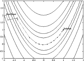
The Levenberg-Marquardt method therefore uses a search direction that is a cross between the Gauss-Newton direction and the steepest descent direction. This is illustrated in Figure 10-1, Levenberg-Marquardt Method on Rosenbrock's Function. The solution for Rosenbrock's function converges after 90 function evaluations compared to 48 for the Gauss-Newton method. The poorer efficiency is partly because the Gauss-Newton method is generally more effective when the residual is zero at the solution. However, such information is not always available beforehand, and the increased robustness of the Levenberg-Marquardt method compensates for its occasional poorer efficiency.
Figure 10-1. Levenberg-Marquardt Method on Rosenbrock's Function
For an animated version of this figure, enter bandem at
the MATLAB® command line.