Requirement: Add a database.
- Open the process Diffusion and Tracking => Import => Generic Diffusion Importation.
- Select input data with
 icon for the parameter files: file or files containing the T2 volume and the diffusion volumes: data_unprocessed/sujet01/diffusion/sujet01_raw_diffusion_o041.ima.
 - Select also the second input parameter bValuesAndOrientations, a text file giving the bvalue and orientation for each volume: data_unprocessed/sujet01/diffusion/diffusion_o041.txt
- Describe Output parameter with
 icon. You have to fill in several information fields for this data:
- Select a format: for example NIFTI-1 image; the image will be converted to this format in the database directory.
- Type a name for the protocol attribute, for example demo.
- Type a name for the subject, for example subject01.
- A suggested item appears in the right panel. Click Ok button to accept.
- The distorsions are already corrected in the demo data, so select True for the dw_already_corrected parameter.
- Click on Run button to start the process.

Note
There are other importation processes, specific to an acquisition sequence and/or a scanner. They may avoid having to give the directions list. But if there is no specific importation process for your case, you can still use the generic one or create your own importation process.Requirement: Import diffusion data.
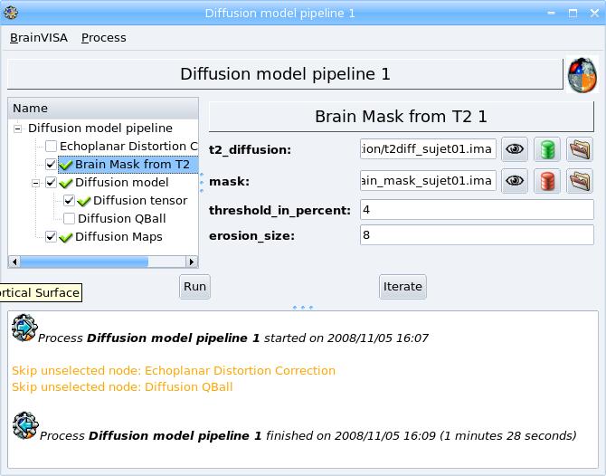
To run the pipeline:
- Open the process Diffusion and tracking => Diffusion model pipeline.
- Select the input T2 MRI with the
 icon: subject01.
 - All the other parameters are automatically filled in.
- Select the type of model you want to compute. Two models are available Diffusion Tensor (DTI) and QBall. The default model is DTI. The computation of this model is faster but is also more simple and do not represent the fibers crossings for example.
- In Brain mask from T2 step, set the value of erosion_size parameter to 8.
- Click Run button to start the process.
- Visualize the results.
Note
In this example, the Echoplanar Distortion Correction step has been automatically unselected because input data are already corrected.
Requirement: Diffusion model pipeline.
In this step, we will do a white matter fascicles tracking. The algorithm needs regions of interest (ROI) defined as starting points for the tracking. The starting points can be in the form of a mask or a ROI graph. That is why the first step of the pipeline offers to draw regions of interest.
First, we will do the tracking from existing ROIs which we will import in database. To do so, we will use a generic importation process that enable to import any type of data.
- Open the process Data management => Import => GeneralImport .
- Select the ROI graph as input data with icon: data_unprocessed/sujet01/diffusion/sujet01_tracking_roi.arg
- Select the type of data to import with the parameter data_type: here Tracking regions graph.
- Describe the output parameter with icon. Enter a value for protocol and subject attributes: the same values you enter for diffusion data importation.
- Select the matching T2 value for the copy_referential_of parameter to assign this referential to the imported data.
- Start the process.
Now, let us use these regions as the starting points of the tracking algorithm. Open the process Diffusion and tracking => Fascicles Tracking Pipeline.
- Select the T2 image in the database with icon for the t2_diffusionparameter.
- Select the regions of interest previously imported for the starting_points parameter.
- Start the pipeline.
- Visualize the results.
To draw ROIs:
- Select only the process ROI drawing in the pipeline.
- Select the image on which you want to draw the regions with the icon and select for example the RGB map.
- If you want to keep several ROI graphs and several tracking results, don't forget to change the tracking_session attribute of the output data. Thus, the different tracking sessions will be stored in different directories. With the icon of the ROI parameter, enter a value for the protocol, subject (the same as for the input data) and session attribute, for example session1.
- Start the process. It opens the Anatomist ROI panel. Selects the region region in Anatomist ROI panel, adjust the brush parameters as you wish in the paint tab. Now, you can draw the regions. When this is done, save the graph trhought the menu ROI managment => File => Save As. The ROI graph is now stored in database and can be used as the starting points of the tracking algorithm.
Note
The white matter fascicles are stored in file with the extension .bundles.
It is possible to use regions drawn from a T1 MRI but in this case we have to be careful with the referential, the T1 MRI and the T2 MRI must be registered or we would need a transformation between the two images, that can be given to the tracking algorithm through the starting_point_transformation parameter.
This step enables to refine the fascicles selection: for example, it is possible to cut the set of fascicles got in previous step into several subsets according to the crossed ROIs.
To cut the set of fascicles :
- Open the process Diffusion and Tracking => Fascicles Tracking Pipeline.
- Select the T2 image in the database with icon for the t2_diffusionparameter.
- Select only the process Diffusion Bundles Transformation.
- Click on this step.
- Select the ROI graph for the split_regions parameter.
- Start the process.

Note
It is possible to define rules for fascicles selection. Look at the inline documentation for the process Diffusion and Tracking => Tracking pipeline components => Diffusion Bundles Transformation for more details.
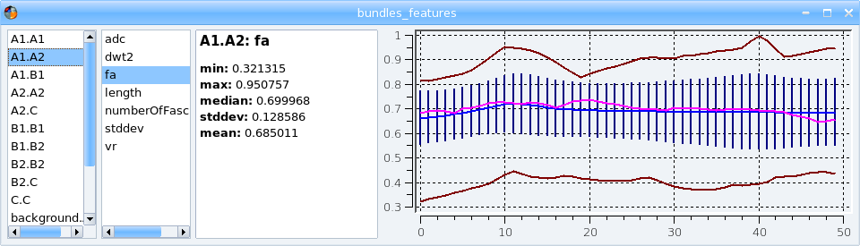
This process computes some quantitative information for each input bundle. The results are stored in a .features file.
To start the analysis:
- In the Fascicles Tracking Pipeline Diffusion, select only the step Diffusion Bundles Analysis step.
- Fill in its parameters.
- Start the process.

To visualize the .features results file with its dedicated viewer, click on the  icon.
icon.